compcogneuro 翻訳ページ

compcogneuro/book: の学習

このページは外部資料の日本語訳です。原文の見出し順と本文順を保ち、コード・URL・出典表記はできるだけ原形のまま残しています。

種別

翻訳資料

更新日

2026-05-20

対象

外部資料を日本語で原文順に読みたい読者

目安

原文量に依存

確認メモ

機械翻訳をベースにした日本語訳です。実装手順や引用は必ず原典も確認してください。

出典とライセンス

原典: https://github.com/compcogneuro/book/blob/main/chapter-04.md

ライセンス: CC BY 4.0。このページは日本語翻訳であり、変更点は翻訳とサイト内整形です。

bibfile: ccnlab.bib —

の学習

私たちはどうやって読み書き、計算、スポーツを学ぶのでしょうか?ニューラルネットワークでの学習は、送信ニューロンと受信ニューロンの局所的な活動パターンに応じて、シナプスの重みを変更することになります。前の章で強調したように、これらのシナプスの重みは個々のニューロンが何を検出するかを決定するものであり、したがってニューロンとネットワークの動作を決定するための「重要」なパラメーターです。

言い換えれば、あなたが知っていることはすべて、シナプス重みのパターンにエンコードされており、これらはあなたが経験したあらゆる経験によって形成されています（その経験によってニューロンが十分に活性化されている限り）。それらの経験の多くはそれほど強い痕跡を残さず、脳の大部分では個々の経験の痕跡がすべて混ざり合っているため、それらをはっきりと思い出すのは困難です（実際、この混合が全体的な知性にとって非常に有益であることが記憶の章でわかります）。しかし、それにもかかわらず、それぞれの経験はある程度の学習を促進します。この章の大きな課題は、個々のニューロン間の活動パターンの単なる影響がどのようにして積み重なり、大きなことを学習できるようになるのかを解明することです。

生物学的には、シナプス可塑性 (学習によるシナプスの重みの変更) が広範囲に研究されており、現在では神経活動の結果として起こる詳細な化学プロセスについて膨大な量がわかっています。ここでは、複数のレベルの詳細を提供します (スパイクタイミング依存可塑性 (STDP) についての説明を含みます。これは、この分野の多くの研究者の想像力を魅了しています)。しかし、高レベルの話は非常に単純です。シナプスの両端の神経活動 (神経発火の送受信) の全体的なレベルが、NMDA チャネルを介したカルシウムイオン ($Ca^{++}$) の流入と、シナプスの重みの変化を促進します。これらは、特定のシナプスに関連付けられた 樹状突起スパイン の シナプス後 $Ca^{++}$ のレベルによって駆動されます。 $Ca^{++}$ のレベルが低いとシナプスが弱くなり、レベルが高いとシナプスが強くなります。

計算的には、多くの異なる計算目標を達成するためにシナプス重みの変化を駆動できる、多くの異なる方程式のセットが開発されています。これらのうち、生物学が実際に行っていることに対応するものはどれですか?それが大きな疑問です。最終的な答えは依然として掴みどころがありませんが、それでも、生物学的データとよく一致し、最も困難な認知タスク（例：物体の読み取りや認識の学習）を解決できる、計算的に非常に有用な形式の学習を実行できる妥当な候補が得られています。

学習には主に 2 つのタイプがあります。

自己組織化学習。環境に関するより長い時間スケールの統計を抽出するため、外界の効果的な内部モデル (つまり、世界でどのような種類のことが確実に発生する傾向があるか – これらを統計的規則性と呼びます) を開発するのに役立ちます。
エラー主導型 学習。期待と結果の間のより迅速な対比を使用してこれらの期待を修正し、世界の偶発的事象についてより詳細で具体的な知識を形成します。たとえば、幼い子供たちは、ハイチェアのトレイから物を押し出すと何が起こるかを学ぶことに際限なく興味を持っているようです。それでも、今度は地面に落ちて大混乱になるでしょうか?正確に何が起こるかについて十分に正確な予想を立てると、それは少し興味を失い始め、他のより予測不可能な事柄が彼らの興味を引き始めます。この例からわかるように、間違い主導の学習は、好奇心、驚き、その他の動機付け要因と密接に結びついている可能性があります。このため、ドーパミン、ノルエピネフリン、アセチルコリンなどの神経調節物質は、さまざまなバージョンの驚き、つまり期待と結果の間に矛盾がある場合に関与しているため、この形式の学習を調節するのに重要な役割を果たしている可能性が高いと仮説を立てています。

興味深いことに、これら 2 つの学習形式の主な計算上の違いは、重要な変数の 1 つが更新される時間スケールに関係しています。自己組織化学習には長い時間スケールにわたる平均化が含まれますが、エラー駆動学習ははるかに高速です。この違いは上記の説明でも強調されており、これらのタイプの学習の違いについての直観の重要な情報源となります。自己組織化学習は、目をかすみ、時間をかけてただ物事を受け入れたときに起こるものですが、エラー主導型学習では、より注意力があり、迅速な神経活動が必要です。この本の残りの部分で使用するフレームワークでは、これらのタイプの学習を 1 つの学習方程式に組み合わせて、私たちがどのように認識、記憶、読み取り、計画を立てるようになるかを探ります。

シナプス可塑性の生物学

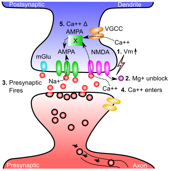
$カルシウムイオン ($Ca^{++}$) が NMDA チャネルを介してシナプス後細胞に侵入し、シナプス可塑性を誘導するための重要なステップ。 1. シナプス後膜電位 ($V_m$) が上昇する必要があります (シナプス後ニューロンのシナプスを横切る AMPA 受容体への興奮性入力と、シナプス後ニューロンの発火時に樹状突起を下って戻ってくる逆伝播活動電位から)。 2. $V_m$ が上昇すると、マグネシウム (Mg+) イオンが NMDA チャネル開口部から排出され、チャネルのブロックが解除されます。 3. シナプス前ニューロンが活動電位を発火させ、グルタミン酸を放出します。 4. グルタミン酸は NMDA 受容体に結合して NMDA 受容体を開き、$Ca^{++}$ の侵入を可能にします (ステップ 2 に従ってブロックが解除されている場合のみ)。 5. シナプス後脊椎における $Ca^{++}$ の濃度は、セカンドメッセンジャーシステム (X で示す) を駆動し、AMPA 受容体の有効性を変化させ、それによってシナプスの重みを変化させます。 $Ca^{++}$ は、電位依存性カルシウムチャネル (VGCC) からも侵入できます。VGCC は、シナプス後 $V_m$ レベルのみに依存し、活動を送信しません。これらは、$Ca^{++}$ レベルへの寄与が弱いです。$

学習は、2 つのニューロンを接続するシナプスの全体的なシナプス効果を変えることに相当します。シナプスには多くの可動部分があり (ニューロン の章を参照)、そのうちの 1 つが、全体的な有効性を変化させる重要な要因となる可能性があります。あなたはいくつ思いつきますか？重要な因子の探索は、シナプス可塑性に関する研究の初期段階を支配しており、放出されるシナプス前神経伝達物質の量から、シナプス後AMPA受容体の数と有効性、さらにはシナプス前成分と後成分の配列などのより微妙なものや、複数のシナプスのクローニングなどのより劇的な変化に至るまで、さまざまな要因の関与の証拠が長年にわたって発見されてきました。しかし、長期にわたる学習変化の支配的な要因は、シナプス後 AMPA 受容体の数と有効性であると考えられます。

[@fig:fig-ltpd-synapse] は、AMPA 受容体の有効性の変化を引き起こす一連のイベントにおける 5 つの重要なステップを示しています。 NMDA 受容体とカルシウムイオン ($Ca^{++}$) が中心的な役割を果たします — NMDA チャネルにより、$Ca^{++}$ がシナプス後脊椎に入ることが可能になります。 $Ca^{++}$ は通常、体内のすべての細胞において細胞機能の調節に重要な役割を果たしており、ニューロンでは一連の化学反応を引き起こすことができ、最終的にはシナプス内で機能する AMPA 受容体の数を制御します。これらの反応の詳細については、学習の詳細な生物学に関する付録の章を参照してください。 $Ca^{++}$ がシナプス後細胞に到達するために必要なものは次のとおりです。

すべての興奮性シナプス入力が細胞に流入するため、シナプス後膜電位 ($V_m$) が上昇する必要があります。この $V_m$ レベルの最も重要な要因は、実際には 逆伝播する活動電位 です。ニューロンが活動電位を発火させると、活動電位は軸索から前方に進むだけでなく、(樹状突起に沿ったアクティブな電圧感受性の $Na^+$ チャネルを介して) 樹状突起に沿って後方にも下降します。したがって、ニューロン全体がいつ発火したかを知ることができます。これが計算上非常に役立つことがわかります。
$V_m$ が上昇すると、マグネシウムイオン ($Mg^+$) が NMDA チャネルの開口部から反発され (正電荷が互いに反発し)、チャネルのブロックが解除されます。
シナプス前ニューロンは活動電位を発火させ、グルタミン酸神経伝達物質をシナプス間隙に放出します。
グルタミン酸は NMDA 受容体に結合し、NMDA 受容体を開いて $Ca^{++}$ イオンがシナプス後細胞に流入できるようにします。これは、NMDA もブロック解除されている場合にのみ発生します。後で説明するように、シナプス前およびシナプス後活動の両方に対する NMDA の依存性は、学習の性質を知るための初期の重要な手がかりの 1 つでした。
シナプス後脊椎における $Ca^{++}$ の濃度は、最終的に AMPA 受容体の数と有効性を変化させる複雑な化学反応を促進します。これらの AMPA 受容体はニューロンに一次興奮性入力駆動を提供するため、AMPA 受容体を変更すると、シナプス後ニューロンに対するシナプス前活動電位の正味の興奮効果が変化します。これが、シナプスの効力、つまり重量を変更することを意味します。

$Ca^{++}$ は、膜電位が上昇した場合にのみ開くカルシウムチャネルである 電位依存性カルシウムチャネル (VGCC) を介してシナプス後細胞に侵入することもあります。ただし、NMDA とは異なり、それらはシナプス前神経活動に「敏感ではなく」、シナプス後活動にのみ依存します。後で説明するように、これは計算上重要な意味を持ちます。 VGCC は NMDA よりも $Ca^{++}$ レベルへの寄与が少ないため、依然として NMDA が支配的なプレーヤーです。

代謝型グルタミン酸受容体 (mGlu) も、シナプス可塑性において重要な役割を果たします。これらの受容体はイオンが膜を越えて流れることを許可せず（つまり、イオンチャネル刺激性ではありません）、代わりに神経伝達物質が結合すると直接化学反応を引き起こします。これらの化学反応は、$Ca^{++}$ によって引き起こされる AMPA 受容体の変化を調節する可能性があります。

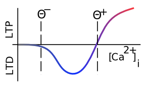
$シナプス可塑性の方向 (LTP = 増加、LTD = 減少) をシナプス後脊椎の $Ca^{++}$ 濃度 (数百ミリ秒にわたって蓄積) の関数として示します。 $Ca^{++}$ のレベルが低いと LTD が発生し、レベルが高くなると LTP が発生します。シータ値で示される閾値レベルは、関数の符号が変化するレベルを表します。$

私たちは、AMPA受容体の有効性の変化について、変化の方向を特定することなく話してきました。 長期増強(LTP)は、AMPA有効性の長期にわたる増加を意味する生物学的用語であり、長期うつ病(LTD)は、AMPA有効性の長期にわたる減少を意味します。長い間、研究者は主に LTP (一般に誘発が容易である) に焦点を当てていましたが、最終的にはシナプス可塑性の両方の方向が学習にとって同等に重要であることに気づきました。 [@fig:fig-ltp-ltd-ca2] は、この変化の方向がシナプス後脊椎の $Ca^{++}$ の全体的なレベル (少なくとも数百ミリ秒にわたって蓄積される — シナプス可塑性に対する $Ca^{++}$ の影響に関連する時定数はかなり遅い) にどのように依存するかを示しています — 低レベルは LTD を駆動し、高レベルは LTP を生成します。このプロパティは、計算モデルにとって重要です。 $Ca^{++}$ レベルに基づくシナプス可塑性効果の遅延は、シナプスが LTP に至る途中で常に LTD を実行する必要があるわけではないことを意味します。重みが変更され始める前に、$Ca^{++}$ が LTP を駆動するために高レベルに達する時間があります。

Hebbian 学習と NMDA チャネル

有名なカナダの心理学者ドナルド O. ヘブは、機能レベルで学習がどのように機能するかを考えるだけで、発見の何年も前に NMDA チャネルの性質を予測しました。重要な引用は次のとおりです。

残響活動 (または「痕跡」) の持続または繰り返しが、その安定性を高める永続的な細胞変化を誘発する傾向があると仮定しましょう。… 細胞 A の軸索が細胞 B を興奮させるのに十分近くにあり、繰り返しまたは持続的にその発火に関与すると、一方または両方の細胞で何らかの成長プロセスまたは代謝変化が起こり、B を発火する細胞の 1 つとして A の効率が増加します。

これは、一緒に発火し、一緒に配線されるセルとしてより簡潔に要約できます。$Ca^{++}$ が入って学習を促進するには、シナプス前とシナプス後の両方の活動が必要であるため、NMDA チャネルはこのプロセスに不可欠です。神経発火の「偶然」を検出できます。興味深いことに、ヘブは、誰かがヘブの学習原理がNMDA受容体の形で発見されたと告げられたとき、「大したことだ、もうそうなるはずだと分かっていた」という趣旨のことを言ったとされている。

数学的には、ヘビアン学習は次のように要約できます。 $\Delta w = x y$ ここで、$\Delta w$ は、送信アクティビティ x と受信アクティビティ y の関数としてのシナプス重み w の変化です。

学習ルールでこの種の事前事後積が見られると、それはヘビアン学習の一形態として説明される傾向があります。 Hebbian 学習とそのさまざまな一般的なバリエーションの詳細については、Hebbian Learning 付録を参照してください。

以下で詳しく説明しますが、ヘビアン学習のこの最も基本的な形式は非常に限定的です。なぜなら、重みは増加するだけであり (神経活動がスパイクの割合であるため、正の量のみであると仮定すると)、際限なく増加するからです。興味深いことに、Hebb 自身は LTD ではなく LTP のみを検討していたようで、おそらくこれは適切でしょう。しかし、計算モデルでは何の役にも立ちません。物事の計算面に入る前に、生物学におけるもう 1 つの重要な結果について説明します。

スパイクタイミングに依存する可塑性

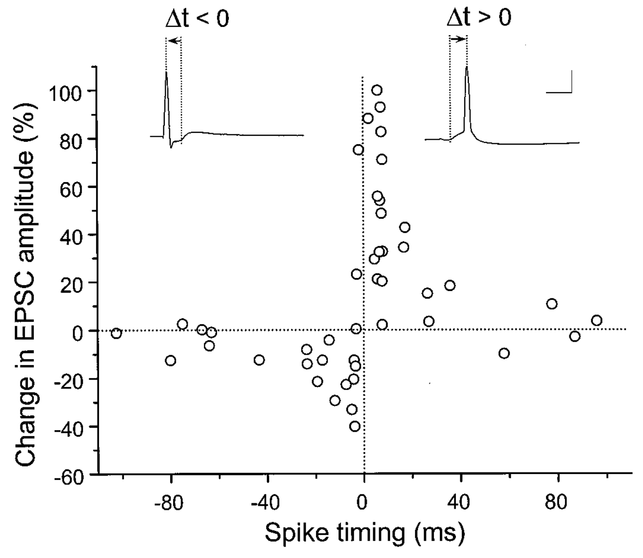
$スパイクのタイミングに依存する可塑性は、シナプス前ニューロンとシナプス後ニューロンの発火の時間的オフセットの観点から実証されました。ポストがプレ ($\Delta t > 0$、右側) の後に発射される場合、重みは増加し、そうでない場合 ($\Delta t < 0$、左側) は重みが減少します。これは、事前から事後までの情報の因果的な流れと一致します。ただし、より複雑なスパイクのシーケンスでは、そのような正確なタイミングが失われ、より一般的な形式の Hebbian のような学習が生じます。 Bi and Poo (1998) から再録。$

[@fig:fig-stdp-bipoo98] は、多くの科学者の想像力を魅了し、広範な計算モデリング作業をもたらした実験 [@BiPoo98] の結果を示しています。この実験は、シナプス前ニューロンとシナプス後ニューロンの間の正確な発火順序がシナプス可塑性の兆候を決定し、シナプス前ニューロンがシナプス後ニューロンより前に発火した場合にはLTPが生じ、そうでない場合にはLTDが生じることを示した。この スパイクタイミング依存可塑性 (STDP) は、シナプス後ニューロンの駆動におけるシナプス前ニューロンの 因果的 役割と一致するため、非常に興味深いものでした。特定のプレニューロンが実際にポストニューロンを発火させる役割を果たしている場合、必然的にその前に発火している必要があり、STDP の結果によれば、その重みは強度が増加します。一方、シナプス後細胞の発火に因果関係のない前ニューロンの重みは減少します。ただし、この STDP パターンは、ニューロンが数百ミリ秒 [@ShouvalWangWittenberg10] にわたって絶えず発火し、相互作用する現実的なスパイク列にはうまく一般化できません。それにもかかわらず、STDP データは、シナプス可塑性の計算モデルに対する有用な厳密なテストを提供します。私たちは、より基本的な生物学的に根拠のあるシナプス可塑性メカニズムを使用した詳細なモデルに基づいて学習方程式を作成しています。このモデルは、これらの STDP 結果 [@UrakuboHondaFroemkeEtAl08] を確実に捉えていますが、発火率のレベルで考慮すると、非常に単純な学習方程式になります。

拡張された対照的アトラクター学習 (XCAL) モデル

このテキストの残りの部分でモデルに採用する学習関数は、eXtended Contrastive Attractor Learning (XCAL) ルールと呼ばれます。（この命名の根拠は後ほど明らかになります）。この学習関数は、ボトムアップ (詳細な生物学的考察によって動機付けられる) アプローチとトップダウン (計算上の要望によって動機付けられる) アプローチの収束を通じて導き出されました。ボトムアップ導出では、[@UrakuboHondaFroemkeEtAl08] によって、既知のシナプス可塑性メカニズムの非常に生物学的に詳細な計算モデルから経験的学習関数 (XCAL dWt 関数と呼ばれる) を抽出しました (詳細については、学習の詳細な生物学 に関する付録の章を参照してください)。彼らのモデルには、シナプス可塑性に関与する主要な生物学的プロセスのすべてについて、経験的測定に基づいた詳細な化学速度パラメータや拡散定数などが組み込まれています。私たちは、以下に示す、そこから現れる単純な区分線形関数を使用して、モデルの信じられないほどの複雑さ (そして、できれば脳内の実際のシナプス可塑性メカニズムの複雑さ) の多くを捉えます。この XCAL dWt 関数は、[@fig:fig-ltp-ltd-ca2] に示されている関数によく似ており、$Ca^{++}$ レベルに対するシナプス可塑性の依存性をプロットしています。また、BCM 学習関数 (自己組織化学習 セクションで詳しく説明されています) にもよく似ています。

トップダウンのアプローチは、BCM 学習機能の背後にある重要なアイデアを活用しています。これは、LTP と LTD を導き出すために必要なアクティビティ量を決定するための 変動しきい値 の使用です。具体的には、閾値は特定の値に固定されるのではなく、長期間にわたって対象となるシナプス後ニューロンの平均活動レベルの関数として調整され、恒常性の動態が得られます。比較的活動的ではなかったニューロンは、より低い活動レベルでシナプスの重みを容易に増加させることができるため、「ゲームに戻る」ことができます。逆に、比較的過剰に活動していたニューロンは、シナプスの重みを減らし、「すべてを独り占めするのをやめる」可能性が高くなります。

以下で説明するように、この関数は有用な 自己組織化 学習に貢献し、さまざまなニューロンが特定の環境における統計構造の異なる側面を抽出するようになります。しかし、純粋な自己組織化メカニズムは、学習できる内容が非常に限られており、統計的一般性 (たとえば、動物は 4 本の足を持つ傾向がある) によって動かされており、生物が直面する機能的要求により実際的に適応することができません。たとえば、いくつかのオブジェクトは他のオブジェクトよりも認識することが重要です（たとえば、友人と敵は重要ですが、ランダムな植物やゴミや瓦礫はそれほど重要ではありません）。

これらのより実用的な目標を達成するには、統計パターンを分類するだけでなく、特にエラーを修正することに焦点を当てたエラー駆動型の学習が必要です。幸いなことに、同じ変動しきい値メカニズムを使用して、より高速な時間スケールでしきい値を適応させることにより、同じ全体的な数学的枠組み内でエラー駆動学習を実現できます。この場合、アクティビティ状態が直前のレベルよりも大きい場合は重みが増加し、逆に、アクティビティレベルが以前の状態と比較して低下した場合は重みが減少します。したがって、最近の活動レベル (しきい値) は期待を反映しており、その後、その差 (または「誤差」) が学習を促進する実際の **結果 ** と比較されると考えることができます。どちらの形式の学習 (自己組織化とエラー駆動型) も非常に有用であり、まったく同じ数学的フレームワークを使用するため、これらを、異なる時間スケール (最近および長期の平均) にわたる統合されたアクティビティレベルを反映する 2 つのしきい値を持つ 1 つの方程式セットに統合します。

次に、XCAL dWt 関数 (dWt = 重みの変化) について説明し、その後、この関数が両方の形式の学習をどのように捉え、その後それらを単一の統一フレームワークに統合するかを説明します (その名前についてのお約束の説明も含まれます!)。

XCAL dWt 関数

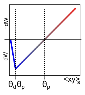
$XCAL dWt 関数。送信ニューロンの短期平均アクティビティ (x) と受信ニューロン (y) の積の関数として、シナプス重み変化 (dWt) の方向と大きさを示します。この量は、シナプス後 $Ca^{++}$ のレベルに対する単純な数学的近似であり、神経活動の送信と受信の両方に対する NMDA チャネルの依存性を反映しています。この関数は、詳細な生物物理学的な Urakubo、Honda、Froemke、Kuroda (2008) モデルから、広範囲の送受信スパイキングパターンの関数として現れるシナプス重みの変化挙動に区分的線形関数を当てはめることによって、そのモデルから直接抽出されました。$

[@UrakuboHondaFroemkeEtAl08] モデルから抽出された XCAL dWt 関数を [@fig:fig-xcal-dwt-fun] に示します。まず、この関数への主な入力は、送信ニューロンと受信ニューロンの活動の発火率と活動期間を反映する 総シナプス活動 です。送信アクティビティレート x と受信アクティビティレート y を持つレートコードモデルの数学的用語では、これは上で説明した「ヘビアン」積になります。 $\Delta w = f_{xcal} \left( x y, \theta_p\right)$ ここで、$f_{xcal}$ は、[@fig:fig-xcal-dwt-fun] で示される区分線形関数です。重みの変化は、追加の動的しきい値パラメータ $\theta_p$ にも依存します。これは、重みの変化が負から正に切り替わる点、つまり重みが逆符号に変化する点を決定します。完全を期すために、この関数の数式を次に示します。ただし、図に示す形状を理解するだけで十分です。 $f_{xcal}(xy, \theta_p) = \begin{整列} (xy - \theta_p) & \mbox{if} \; xy > \theta_p \theta_d \\ -xy (1 - \theta_d) / \theta_d & \mbox{その他の場合} \end{整列}$ ここで、$\theta_d = .1$ は、関数の方向が反転する点 (つまり、重み減少領域内でゼロに戻る点) を決定する定数です。— この反転点は $\theta_p \theta_d$ で発生するため、動的な $\theta_p$ 値に従って適応されます。

前のセクションで述べたように、送信ニューロンと受信ニューロンの両方の活動に対する NMDA チャネルの依存性は、この単純な Hebbian 積で要約でき、細胞内 $Ca^{++}$ のレベルはこの値を反映している可能性があります。したがって、XCAL dWt 関数はこれらの点で非常に理にかなっています。XCAL dWt 関数は、実証研究から確立され、長い間他の理論モデルによって仮定されてきた $Ca^{++}$ の関数としての重量変化の定性的性質を反映しています。 Urakubo モデルは、$Ca^{++}$ レベルおよび関連する LTP/LTD に対するシナプス前/後スパイクタイミングの詳細な影響をシミュレートしますが、発火率のレベルでのこれらの影響から現れるのは、より単純な基本関数です。

この基本的な XCAL dWt 関数は、学習関数として、単純な Hebbian 関数に比べていくつかの利点がありますが、その中心にある「pre * post」用語による基本的な性質を共有しています。たとえば、dWt 関数の形状により、重みは増加だけでなく減少もしますが、ヘビアン関数では重みが増加するだけです。しかし、(アクティビティレベルがしきい値を超えることが多い限り) 重みが際限なく増加するという問題がまだあります。次のセクションでは、他のトップダウンの計算動機による変更により、この基本形式を維持しながら、より強力な学習形式が得られることを見ていきます。

自己組織化学習: 長期スケールと BCM モデル

!【BCM学習機能の形状。 XCAL dWt 関数 ([@fig:fig-xcal-dwt-fun]) と $Ca^{++}$ ([@fig:fig-ltp-ltd-ca2]) の関数としてのシナプス可塑性の両方に対する定性的形状の類似性に注目してください。](figures/fig_bcm_function.png)

主な計算動機は、[@BienenstockCooperMunro82] で始まる一連の学習関数から来ており、これらのイニシャルが関数名 BCM の由来になっています。 (興味深いことに、ノーベル物理学賞受賞者のレオン・クーパーも、超伝導のBCS理論の「中心人物」でした)。 BCM 関数はヘビアン学習の修正形式であり、時間の経過とともに個々のニューロンの発火が多すぎたり少なすぎたりしないようにする興味深い 恒常性 メカニズムが含まれています。 $\Delta w = x y \left(y-\theta\right)$ ここでも x = 送信アクティビティ、y = 受信アクティビティ、$\theta$ は受信ニューロンのアクティビティの 長時間平均を反映する 浮動しきい値です。 $\theta = \langle y^2 \rangle$ ここで、$\langle \rangle$ は期待値または平均を示し、この場合は受信ニューロンの活性化の 2 乗を示します。

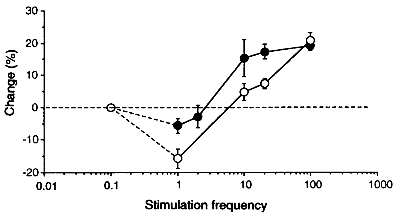
[@fig:fig-bcm-function] は、この関数がどのようなものであるかを示しています。この形は、かなり見慣れたものになっているはずです。実際、BCM 学習関数が $Ca^{++}$ ([@fig:fig-ltp-ltd-ca2]) の関数としてのシナプス可塑性の定性的性質を予測していたという事実は、理論的先見性の驚くべき例です。さらに、BCM 研究者らは、BCM がさまざまな行動学習現象をうまく説明し、同等のヘビアン学習メカニズム [@CooperIntratorBlaisEtAl04; @KirkwoodRioultBear96] ([@fig:fig-kirkwood-et-al-96-bcm-thresh]) よりもよく適合していることを示しました。 NMDA 受容体による Ca++ 透過性の修飾など、この変動閾値の基礎となるメカニズムのレビューについては、[@ScottFrank23] を参照してください。

暗所飼育（黒丸）および通常飼育（白丸）ラットからのシナプス可塑性データ。暗所飼育ラットの方がLTPの閾値が低く、BCM浮遊閾値と一致しているようであることを示している。これらの動物のニューロンは、おそらく全体的にはるかに活性が低いため、その閾値が下がり、LTD と比較して LTP を示す可能性が高くなります。 Kirkwood、Rioult、および Bear (1996) から転載。

BCM は通常、入力パターンが与えられた場合に各ニューロンの活性化値が 1 つだけ存在する単純なフィードフォワードネットワークに適用されます。しかし、時間の経過とともに活動状態が継続的に進化するアトラクターダイナミクスを備えた、より現実的な双方向接続システムでは、重みはどのように更新されるべきでしょうか? BCM 方程式の XCAL バージョンでは、この問題に直面します。 $\Delta w = f_{xcal}( xy, \langle y \rangle_l) = f_{xcal}( xy, y_l)$ ここで、xy は 短期平均シナプス活動 (数百ミリ秒の時間スケール – シナプス可塑性を駆動する $Ca^{++}$ 蓄積の時間スケール) であると理解されており、より正式には次のように表現できます: $\langle xy \rangle_s$、$y_l = \langle y \rangle_l$ はシナプス後ニューロンの 長期平均活動 (つまり、本質的には BCM と同じですが、二乗はありません)。これは、XCAL 関数の $\theta_p$ 浮動しきい値の役割を果たします。

かなりの実験を行った結果、$y_l$ フローティングしきい値を計算する次の方法が、しきい値を制御し、全体的な最適な学習ダイナミクスを実現する最適な機能を提供することを発見しました。 $\begin{整列} \mbox{if} \; y > .2 \; \mbox{その後} \; y_l & = y_l + \frac{1}{\tau_l} \left( \mbox{max} - y_l \right) \\ \mbox{else} \; y_l & = y_l + \frac{1}{\tau_l} \left( \mbox{min} - y_l \right) \end{整列}$

これにより、受信ユニットのアクティビティが基本アクティビティしきい値の 0.2 を超えるかどうかに応じて、最大または最小の極値への適切に制御された指数関数的なアプローチが生成されます。積分 $\tau_l$ の時定数はデフォルトで 10 です。約 10 回の試行にわたって積分します。詳細については、付録 Leabra の詳細 の章を参照してください。

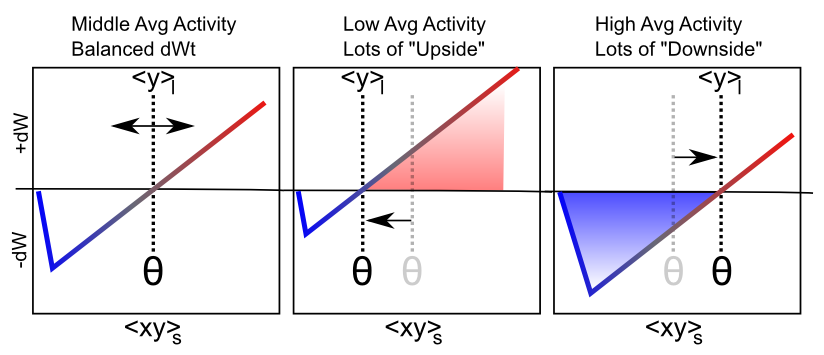
$長期平均受信神経活動 $\langle y \rangle_l$ の関数としての変動閾値が恒常性挙動をどのように駆動するか。平均アクティビティが低いニューロンは、しきい値が低いため、重みが増加する可能性が非常に高くなりますが、平均アクティビティが高いニューロンは、しきい値が高いため、重みが減少する可能性が非常に高くなります。$

[@fig:fig-xcal-bcm-selforg-learn] は、この学習メカニズムの主な定性的動作を示しています。受信者の長期平均アクティビティが低い場合、しきい値は下降し、そのため、短期シナプスアクティビティ値が正の重み変化領域に入る可能性が高くなります。これにより、全体的なシナプスの重みが増加する傾向があり、その結果、ニューロンが将来的に活動しやすくなり、恒常性の目的が達成されます。逆に、受信者の長期平均アクティビティが高い場合、閾値も高くなるため、短期的なシナプス活動によって重みが増加するよりも減少する可能性が高くなります。これにより、これらの過剰に活動するニューロンが 1 ～ 2 段階低下し、最終的にネットワークの活動を支配することがなくなります。

自己組織化学習ダイナミクス

より公平な方法で神経活動を周囲に分散させるこの能力は、ニューロンが表現する対象の空間をより効率的かつ効果的にカバーできるようになるため、自己組織化学習にとって重要であることが判明しました。その理由を知るために、自己組織化学習ダイナミクスの重要な要素を次に示します (これが実際にどのように機能するかを実際に理解するには、後続のシミュレーションの探索を参照してください)。

抑制性競合 — 最も強く駆動されたニューロンのみが抑制性閾値を超えて活動化できます。これらは、現在のシナプス重みが現在の入力パターンに最もよく適合 (「検出」) するものです。
金持ちはさらに金持ちになる 正のフィードバックループ — 学習関数の性質により、実際にアクティブになるニューロンのみが学習できます (受信者のアクティビティ y = 0 の場合、xy = 0 もあり、XCAL dWt 関数は 0 で 0 になります)。したがって、現在の入力をすでに最もよく検出しているニューロンが、これらの入力を検出する能力をさらに強化することになります。これは、ヘブの学習関数が「エングラム」を強化する必要がある理由についてヘブが得た重要な洞察です。
ホメオスタシス 正のフィードバックループのバランスを保つ — チェックしないままにしておくと、富裕層から富裕層へのダイナミクスが最終的に少数の単位ですべてを支配することになり、その結果、すべての入力が 1 つの役に立たない広すぎるカテゴリ (「すべて」) に分類されてしまいます。 BCM の恒常性メカニズムは、活動性の高いニューロンの浮動しきい値を上げ、最も優先される入力パターンを除くすべてのニューロンの重みを減少させ、バランスを回復することで、これに対抗するのに役立ちます。同様に、活動性の低いニューロンは正味重量の増加を経験し、より効果的に参加し、競争するようになり、その結果、独特の特徴を表すようになります。

最終的な結果は、統計的規則性を包含する体系的なカテゴリを備えた、さまざまな入力パターンの空間を比較的均等にカバーする一連の神経検出器の開発です。たとえば、猫は牛乳が好きで、犬は骨が好きです。これは、猫と牛乳、犬と骨の信頼できる共起を観察するだけでわかります。この種の信頼できる共起のことを「統計的規則性」と呼びます。 Hebbian スタイルの学習メカニズムが共起パターンを捕捉する理由の非常に簡単な説明については、Hebbian Learning に関する付録の章を参照してください。これは実際には、「一緒に点火するものは一緒に配線する」という基本的な格言の変形にすぎません。

学習率

上記の方程式には、学習率 という重要な要素が欠けています。通常、このパラメータを表すにはギリシャ語のイプシロン $\epsilon$ を使用します。これは単に重みの変化率を乗算するものです。 $\Delta w = \epsilon f_{xcal}( xy, y_l)$

したがって、イプシロンが大きいほど重みの変化が大きくなり、学習が速くなることを意味し、値が小さいほどその逆になります。学習率の一般的な開始値は 0.04 で、時間の経過とともに学習率が低下することがよくあります (これは脳にも当てはまります – 若い脳は古い脳よりもはるかに柔軟です) – これにより、通常、全体的な学習が最速になり、最終的なパフォーマンスが最高になります。

多くの研究者（および製薬会社）は、学習速度が速いほど良いという潜在的に危険な考えを持っており、学習速度を効果的に高めて、たとえばラットがある種の標準的なタスクを通常よりも早く学習させるさまざまな薬が開発されています。しかし、実際には学習速度が遅いことには非常に重要な利点があることが記憶の章でわかります。具体的には、学習速度が遅いほど、システムは学習に より多くの統計 を組み込むことができます。学習率は、エクスペリエンスが平均化される有効な時間枠を決定します。また、学習速度が遅いほど、時間枠が長くなり、より多くの情報を統合できるようになります。したがって、学習速度を遅くすると、より賢く学習できるようになります。ただし、当然のことながら、この賢い学習の結果が実際の行動に影響を与えるまでには、はるかに長い時間がかかるというトレードオフがあります。人間は非常に長期にわたる発達学習の期間において独特であるため、給料を稼ぎ始める前に多くのことを学ぶことができると多くの人が主張しています。これにより、悪影響をあまり受けずに、学習速度をかなり遅くすることができます。

自己組織化学習の探求

このダイナミクスを確認する最良の方法は、計算による探索です。 CCNシムズから self_org シミュレーションを開き、そこからの指示に従います。

エラー主導型学習

自己組織化学習は非常に便利ですが、学習できる内容の種類が大幅に制限されていることがわかります。一般性を抽出するのには最適ですが、特定の複雑なパターンを学習する場合にはあまり役に立ちません。このようなより困難なタイプの問題を学習するには、エラー駆動型の学習が必要です。直感的には、エラー駆動学習は、「生の信号」ではなく「差分」に基づいて学習を推進するため、はるかに強力です。違い (エラー) は、問題を解決するために何をする必要があるかをより正確に示します。生の信号 (神経活動の全体的なパターン) はそれほど有益ではありません。森に圧倒されて木々を見失いがちです。まず最初にエラー駆動学習を機能させる方法を理解した後で、より具体的な例を見ていきます。

まずは、[@WidrowHoff60] によって開発された、エラー駆動学習の最も単純な形式である デルタルール から始めます。 $\Delta w = x (t - y)$ これは、前に示した単純なヘビアン学習ルールと直接比較できます。 $\Delta w = x y$ これは、$y$ レシーバーアクティベーションを差分 (デルタ) または エラー 用語 $(t-y)$ に置き換える方法を示しています。ここで、$t$ は 生成されるはずだった *ターゲット アクティベーションであり、$y$ は 実際に生成されたアクティベーションです。実際の活性化がターゲットと等しい場合、このエラー値 $(t-y)$ はゼロであり、さらに、ターゲットと等しくない場合に エラーを修正するためにシナプスの重みを調整する方法を正確に示します。実際のアクティベーション $y$ が $t$ と比較して低すぎる場合は、重みが増加し、高すぎる場合はその逆になります。

対照的に、Hebbian 学習ルールは、特定のターゲットの状態に関係なく、重みを増やすだけです。つまり、あらゆる種類のターゲット、望ましい動作 (活性化) を単純に考慮しません。 Hebbian ルールの $y$ 値をターゲット値 $t$ に置き換えることができ、それは機能するかもしれませんが、実際には一般的に機能しないことが少しわかります。実際には、生のアクティベーションではなく、エラーの関数として学習する必要があります。

興味深いことに、デルタルールには、ヘビアン方程式とよく似た送信ユニットのアクティブ化 $x$ が含まれており、これは、実際にアクティブな送信ユニットのエラーに対する クレジット (または責任) を割り当てるのに不可欠であることがわかります。これらのユニットについては、シナプスの重みの変更が実際に次回異なる結果をもたらすものであり、アクティビティレベルに比例して重みを調整することで、このロジックの段階的な形式 (最もアクティブな送信ユニット) が提供されます。最大限の称賛や非難を得ることができます）。これについてのもう 1 つの「ヘビアン」な考え方は、生の出力アクティベーションを関連付けるのではなく、送信アクティベーションをエラーに 関連付けている ということです。この特性の専門用語は 単位割り当て であり、より一般的に学習アルゴリズムの重要な機能です。

エラー駆動学習の生物学的基礎: より高速な時間スケールの変動しきい値

$中期平均シナプス活動 $\langle x y \rangle_m$ の関数としての変動しきい値がどのように誤差駆動学習を生み出すことができるか。この中程度の時間枠は、次に何が起こるかについての期待をコード化する神経活動のパターンの発達を反映しています。最も最近の短期的なシナプス活動 (学習を促進する) は、次に起こったことの実際の結果を表します。 dWt 関数は (ほぼ) 線形であるため、結果と期待値の差が効果的に計算されます。定性的には、結果によってニューロン集団が予想よりも大きく活性化された場合、対応する重みは増加しますが、結果の結果として活動状態が低下したニューロンの重みは減少します。これは、低い期待値と高い期待値の場合で上に示されています。$

ヘブ学習則からは一見単純なステップのように見えますが、エラー駆動学習は生物学的な観点から多くの重要な課題をもたらします。たとえば、そもそも目標値はどこから来るのか、生物学的なシナプスはデルタ則のようなものをどのように計算できるのかなどです。ターゲット信号の性質については後ほど詳しく説明しますが、今のところ、予測または期待のようなものを表す神経活性化 $y$ という観点から考えることができ、ターゲットは実際の結果、つまり実際に何が起こるかということです。

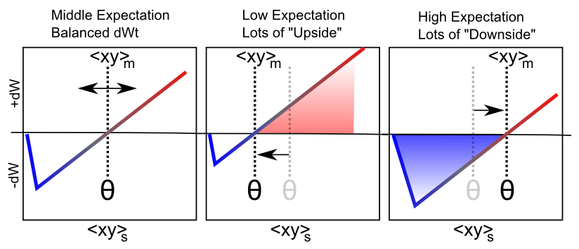
この場合、期待から結果までの自然な時間の流れがあり、XCAL 学習 ([@fig:fig-xcal-bcm-err-learn]) の BCM のような自己組織化の側面の変動しきい値特性を利用することで、2 番目の質問についてより具体的に考えるのに役立ちます。具体的には、浮動しきい値を計算するためのタイムスケールを高速化します (また、受信機の活動だけでなくシナプスの活動も反映させます)。 $\Theta_p = \langle xy \rangle_m$ $\begin{整列} \Delta w & = f_{xcal}( \langle xy \rangle_s, \langle xy \rangle_m) \\ & = f_{xcal}( x_s y_s, x_m y_m) \end{整列}$ ここで、$\langle xy \rangle_m$ は 中時間スケールの平均シナプス活動であり、これは約 75 ミリ秒の神経活動にわたって展開される、現在の状況に対する新たな期待を反映していると考えられます。最も最近の短期間 (最後の 25 ミリ秒) の神経活動 ($\langle xy \rangle_s$) は実際の結果を反映しており、ヘビアンの場合の学習を促進するのと同じカルシウムベースの信号です。

シミュレーターでは、結果が確認される前に、ネットワークによってこの期待が表現される期間は、ボルツマンマシン の用語 [@AckleyHintonSejnowski85] に基づいて、マイナスフェーズと呼ばれます。結果が観察される (そしてその結果の影響を反映するために活性化が進化する) 続く期間は、プラスフェーズと呼ばれます。この期待と結果の差が、エラー駆動学習におけるエラー信号を表します (したがって、マイナスとプラスという用語が生まれます。重みの変化を引き起こすために、プラスフェーズの活性化からマイナスフェーズの活性化が減算されます)。

この期待と結果の比較はエラー駆動型学習の基本的な要件ですが、この違いに基づく重みの変更自体が、ニューロンが自分たちがどのフェーズにあるかをどのようにして「認識」するのかという疑問を引き起こします。私たちはこの疑問に対する多くの可能な答えを模索してきましたが、最新のものには、深層と視床の新皮質回路によってサポートされる、内部で生成されたアルファ周波数（10 Hz、100 ミリ秒周期）の期待とそれに続く結果のサイクルが含まれています。 [@OReillyWyatteRohrlich17; @KachergisWyatteOReillyEtAl14]。このフレームワークの主な意味は、処理と学習のタイミングを次のように整理することです。

トライアルは 100 ミリ秒 (10 Hz、アルファ周波数) 続き、4 つの四半期に編成された 1 つの期待、つまり結果の学習のシーケンスで構成されます。
- 生物学的には、深層新皮質層 (5、6 層) と視床には、アルファ周波数 [@BuffaloFriesLandmanEtAl11; @LorinczKekesiJuhaszEtAl09; @FranceschettiGuatteoPanzicaEtAl95; @LuczakBarthoHarris13] での自然振動リズムがあります。これらの層の特定のダイナミクスは、アルファサイクル内の期待と結果のサイクルを組織します。
四半期 は 25 ミリ秒続きます (40 Hz、ガンマ周波数) — 最初の 3 四半期 (75 ミリ秒) は期待/マイナスフェーズを形成し、最後の四半期は結果/プラスフェーズです。
- Biologically, the superficial neocortical layers (layers 2, 3) have a gamma frequency oscillation [@BuffaloFriesLandmanEtAl11], supporting the quarter-level organization.
サイクルは 1 ミリ秒の処理を表し、各ニューロンはニューロンの章で説明されている方程式に従って膜電位を更新します。

XCAL 学習メカニズムは、最新のシナプス活動 (主にプラス相/結果状態によって駆動される) を中時間スケールで統合されたもの (マイナス相とプラス相の両方を効果的に含む) と比較することで、このタイミングと調整します。 XCAL 学習関数は (ほとんど) 線形であるため、短期結果と比較される中期時間枠 (期待状態を含む) にわたるこのシナプス活動と変動しきい値の関連付けにより、それらの差が直接計算されます。 $\Delta w \approx x_s y_s - x_m y_m$ これは、送信アクティベーションが乗算され (2 つの異なる時間平均に分離され)、$y_s$ が結果ターゲット信号 $t$ を表し、$y_m$ が実際のアクティベーション $y$ を表す、上記のデルタルールに非常に似ています。 $\Delta w \approx x (y_s - y_m)$

直感的には、このルールはデルタルールのように動作し、3 つの異なるケースを考慮することでエラー駆動のダイナミクスを詳しく説明できます。最も簡単なケースは、期待値が結果と等しい場合 (つまり、正しい期待値) です。上記の 2 つの項は同じになるため、それらの減算はゼロになり、重みは同じままになります。したがって、完璧を獲得すると、学習を停止します。もしあなたの期待が結果よりも高かったらどうしますか？差は負の数になり、重みが減少するため、次回の期待値が低くなります。直感的には、これは完全に理にかなっています。M. ナイトシャマランのすべての映画が The Sixth Sense と同じくらいクールになるだろうと期待している場合、実際の結果に合わせて重みを減らす必要があるかもしれません。逆に、期待が結果よりも低い場合、体重の変化はプラスになるため、期待が高まります。

このクラスは死ぬほど退屈だと思ったかもしれませんが、おそらく上記の M. ナイトシャマランの言及が面白かったので、今度は体重を少し増やす必要があります。この形式の学習が時間の経過とともに期待と結果の間の差異を最小限に抑えるように機能することが直感的に明らかになることが望ましいです。ここで挙げた例は、価値のある期待からの逸脱（つまり、モーター制御と強化学習の章で詳しく説明するように、物事が予想よりも良くなった、または悪くなった）という観点から投げかけられたものですが、結果が他の種類の期待から逸脱した場合にも同じ原則が適用されることに注意してください。

明示的に時間的な性質があるため、上で定義した明示的なタイミングに加えて、この学習ルールが何を行うかについて考える興味深い方法が他にもいくつかあります。繰り返しになりますが、このルールでは、結果は先行する期待の直後に来ると言われています。これは、直前の時点を含むわずかに長い中期の平均と比較して、短期 (最も直近の) 平均的なシナプス活動に向けて学習させた直接的な結果です。

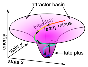
$XCAL エラー駆動学習メカニズムの背後にある中心的なアイデアである、対照的アトラクター学習 (CAL) 原理の図。ネットワークは、セトリングの初期フェーズ (マイナスフェーズ、つまり中時間フレームのアクティブ化平均 $\langle x y \rangle_m$ ) とセトリングの後期フェーズ (プラスフェーズ、つまり短時間フレームのアクティブ化平均 $\langle x y \rangle_s$ ) の対比を学習します。後期フェーズでは、ネットワーク内の全体的な制約がより多く統合されているため、初期フェーズよりも現在の状況の全体的な解釈または表現が「より適切」になっているため、後期フェーズが初期フェーズと比較して「トレーニング信号」として機能することは理にかなっています。$

この学習は、ネットワークの章で説明したアトラクターダイナミクスの観点から考えることができます。具体的には、Contrastive Attractor Learning (CAL) という名前は、ネットワークがアトラクター状態に落ち着くという考えを反映しており、ネットワークが落ち着く最終的なアトラクター状態 (つまり、この場合の「結果」) と、学習を促進するアトラクターに近づくネットワークの活性化軌道との対比です ([@fig:fig-attractor-cal])。短時間スケールの平均は最終的なアトラクターの状態 (「ターゲット」) を反映し、中程度の時間スケールの平均は整定中の軌道全体を反映します。期待に関連付けられた活動のパターンが実際の結果からかけ離れている場合、これら 2 つのアトラクター状態の差は大きくなり、学習によって重みの変化が促進されるため、将来の遭遇では期待が結果をより正確に反映するようになります (環境が信頼できると仮定すると)。 XCAL の X 部分は、離散的な時点で 2 つのアトラクターを明示的に比較する必要がなく、その代わりに、ベースライン比較として整定軌跡全体にわたって拡張された時間平均活動状態を使用することによって、同じ目的が達成されるという事実を単純に反映しています。このような変数は局所的なニューロン活動によって容易にアクセスできるため、生物学的により現実的です。

数学的には、この CAL 学習ルールは、[@NormanNewmanDetreEtAl06; @RitvoTurk-BrowneNorman19] で開発された振動学習関数のより単純なバージョンを表します。

後の情報 (短い時間スケールの平均) が 以前の情報 (中程度の時間スケールの平均) をトレーニングするより一般的な理由もあります。通常、待つ時間が長いほど、情報の質は高くなります。文の初めでは、次に何が起こるかについてある程度の見当が付いているかもしれませんが、文が展開するにつれて、その意味はますます明確になります。この後の情報は、以前の期待を強化するのに役立ち、次回より効率的に物事を理解できるようになります。全体として、XCAL 学習に関するこれらの代替的な考え方は、明示的な結果トレーニング信号を必要とせず、より自己組織化された形式の学習を表しており、エラー駆動型の学習メカニズムに対してより迅速なコントラスト (短い時間と中程度の時間) を使用しています。

続行する前に、このエラー駆動型の変動しきい値の生物学的根拠について疑問に思うかもしれません。 BCM スタイルの変動しきい値とは異なり、それと一致する確かな経験的データがありますが、中程度の時間スケールの平均シナプス活動を反映するために、このより速い時間スケールでしきい値が変化するという考えは、まだ経験的にテストされていません。したがって、これはこの計算モデルの重要な予測となります。それは非常に簡単に計算され、非常に強力な形式の学習をもたらすため、脳がまさにそのようなメカニズムを利用することはもっともらしいように思えますが、それが経験的テストにどのように耐えられるかを見る必要があります。このようなダイナミクスの最初の提案の 1 つは [@LimMcKeeWoloszynEtAl15] から来ており、最近のアクティビティに応じてしきい値が急速に変化する BCM のような学習ダイナミクスを示しています。また、顕著な予期せぬ出来事の際に起こる神経調節の一時的な変化が、シナプス可塑性を修正するのに重要であるという実質的な証拠があり、この種のエラー駆動型の学習メカニズムに機能的に寄与している可能性があります。また、この形式のエラー主導型学習の中心となる、期待と結果の区別の性質と起源に関する別の大きな懸念については、少し後で説明します。

エラー駆動学習の利点

上で述べたように、エラー駆動学習は、自己組織化学習よりもはるかに強力な計算能力を備えています。たとえば、視覚的な外観に基づいてオブジェクトを認識することを学習するという困難な課題でうまく機能するすべての計算モデル (知覚の章を参照) は、エラー駆動型学習の形式を利用しています。さまざまな形式の自己組織化学習を使用するものもありますが、これは補助的な役割を果たす傾向があり、エラー駆動学習がなければモデルは完全に機能しません。エラー駆動学習により、モデルは関連性のある種類のカテゴリ識別を確実に行い、無関係なカテゴリ識別を回避します。たとえば、車の側面図が左を向いているか右を向いているかは、これが車であると判断するのには関係ありません。しかし、車輪の有無は車と魚を見分ける上で非常に重要です。純粋な自己組織化モデルでは、これらの違いは、統計的に非常に信頼でき、入力内の強力な信号である可能性がありますが、人々が関心を持っているカテゴリに対する有用性が異なることを知る方法がありません。

数学的に言えば、エラー駆動型の学習関数の歴史は、科学社会学と、一見単純なアイデアが発展するまでにどのように時間がかかるかを知る興味深い窓を提供します。 バックプロパゲーションに関する付録の章では、デルタルール [@WidrowHoff60] から非常に広く使用されている バックプロパゲーション 学習ルール [@RumelhartHintonWilliams86] まで、誤差駆動学習ルールの導出を通じてこの歴史をたどります。そのサブセクションの冒頭では、誤差駆動学習の XCAL 形式 (具体的にはその CAL バージョン) が逆伝播から直接導出される方法を示し、これにより、なぜ非常に多くの困難な問題を解決できるのかについて数学的に満足のいく説明を提供します。

バックプロパゲーション学習関数の背後にある重要なアイデアは、出力層で発生したエラー信号が以前の隠れ層まで「逆方向に伝播」して、これらの初期層での学習を促進し、ネットワークが直面している全体的な問題を解決できる (つまり、ネットワークが出力層で正しい期待値や答えを確実に生成できるようにする) ということです。これは、システム全体が困難な問題を解決できるようにするために不可欠です。ネットワークの章で説明したように、多くのインテリジェンスは、分類のカスケードステップの複数の層から生じます。これらの介在するすべてのステップが関連するカテゴリに焦点を当てるには、エラー信号がこれらの層全体に伝播し、すべての層で学習を形成する必要があります。

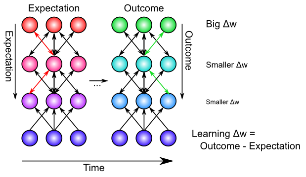
双方向接続によってネットワークの他の部分からの学習信号のバックプロパゲーションがどのように可能になるかについての直観 -- ネットワークのいずれかの部分で期待と結果の間に差異がある場合、ネットワークの他の部分のニューロンは双方向接続を介してその差異を「感じます」。すべてのニューロンは、期待と結果の両方の自身の活性化への影響を経験するため、これら 2 つの時点の間の違いを学習するとき (後のトレーニングで先に)、結果に対する自身の影響、つまり期待誤差について学習することになり、この差に基づいて重みを変更すると、最終的にネットワーク全体の全体的な誤差が最小限に抑えられます。エラーの発生源に近いニューロンが最も多く学習し、この発生源から離れるにつれてエラーは減少します。

生物学的には、モデルの双方向接続により、これらのエラー信号がこのように伝播することが可能になります ([@fig:fig-bidir-backprop-intuition])。したがって、ネットワーク内の任意の場所の変化は、双方向接続を介して後方に放射し (接続のあらゆる方向に)、他のすべての層のアクティブ化状態に影響を与え、これが他の層の学習に影響を与えます。言い換えれば、XCAL は双方向の活性化ダイナミクスを使用してネットワーク全体にエラー信号を伝達しますが、バックプロパゲーションは、通常の活性化の流れとは逆方向に、シナプス接続全体でエラー信号を逆方向に伝播する生物学的にありえない手順を使用します。さらに、XCAL ネットワークは、期待からその後の結果の体験に至る一連のアクティベーション状態を経験し、これら 2 つの状態の違いを学習します。対照的に、バックプロパゲーションでは、結果と期待値の差である単一の誤差 デルタ 値を計算し、この単一の値を接続全体に逆方向に送信します。これら 2 つの異なるものが数学的にどのように同等であるかについては、逆伝播 付録を参照してください。

エラー駆動型学習の探求

CCNシムズの pat_assoc シミュレーションは、基本的な入出力マッピングを学習する単純な 2 層パターンアソシエータのコンテキストで、自己組織化ヘビアンスタイル学習の制限と、エラー駆動学習がこれらの制限をどのように克服するかを示す優れたデモンストレーションを提供します。そのシミュレーションリンクの指示に従って、探索を実行します。

入出力マッピングタスクの 1 つは、2 層ネットワークではエラー駆動学習でも解決するのが「不可能」であることがわかったはずです。次の探索である err_driven_hidden は、隠れ層の追加と強力なエラー駆動学習メカニズムの組み合わせにより、この「不可能な」問題さえも解決できることを示しています。これは、バックプロパゲーションアルゴリズムの計算能力を示しています。

自己組織化学習とエラー主導型学習の組み合わせ

科学者はどちらかの側を強く選択し、自己組織化学習かエラー主導型学習のどちらかが最善の方法であると宣言する傾向がありますが、実際には両方の形式の学習を組み合わせることで多くの利点があります。それぞれの学習形式には、補完的な長所と短所があります。

自己組織化は局所的な発火統計にのみ依存するのに対し、エラー駆動学習は潜在的に遠く離れた領域から来るエラー信号に暗黙的に依存するため、より「堅牢」です。自己組織化により、エラー信号が遠く離れている場合や、まだ一貫性が高くない場合でも、有用な何かを達成できます。
しかし、自己組織化学習は非常に近視眼的でもあり、他の層での学習と連携していないため、「貪欲」になる傾向があります。対照的に、エラー駆動学習はこの調整を実現し、複数のレイヤーにわたる複数のユニットの共同アクションを必要とする問題の解決方法を学習できます。

役に立つかもしれない例えの一つは、エラー主導型学習は社会主義経済学のようなものであるということです。これは、共通の目標を達成するために、さまざまな層や単位がすべて協力する必要があるのに対し、自己組織化型学習は自由市場経済学のようなもので、他者と明示的に調整することなく、どういうわけか社会全体に利益をもたらすローカルで貪欲な行動を強調します。これらの経済的アプローチのトレードオフは、それぞれの形式の学習のトレードオフと似ています。社会主義的なアプローチでは、個々の人々が顔のない巨大な機械の中の小さな歯車にすぎないため、あまりやる気を感じられなくなる可能性があります。同様に、エラー駆動学習に厳密に依存するニューロンは、問題全体の解決に非常に小さく、ある程度「匿名」で貢献するだけで済むため、最終的にはあまり学習しない可能性があります。エラー信号が除去されると (つまり、期待と結果が一致すると)、学習は停止します。純粋なエラー駆動学習に依存するネットワークは、問題全体を解決するために費やされる最小限の労力を反映して、非常にランダムに見える重みを持つことがよくあります。その一方で、より強力な自由市場アプローチは、過剰な正のフィードバックループ (金持ちはさらに金持ちになる) に陥る可能性があり、通常、調整と計画を必要とする長期的で大規模な問題への対処が苦手です。同様に、純粋に自己組織化したモデルは、「表現的富」の分布がより不均一になる傾向があり、困難な問題を解決することはほとんどなく、興味深い統計があれば何でも貪欲にエンコードすることを好みます。興味深いことに、私たちのモデルは、両方のアプローチのバランス、つまり中道アプローチが最も効果的であることを示唆しています。おそらく、この教訓は政治の分野に一般化できるでしょう。

カラフルな例えはさておき、XCAL フレームワーク内で両方の形式の学習を組み合わせる実際の仕組みは、浮動しきい値の 2 つの異なる定義を結合することになります。生物学的には、「ラムダ」パラメーター $\lambda$ を使用して、中期のシナプス余積に対して長期受信機平均 (自己組織化) を重み付けし、2 つのしきい値を組み合わせた加重平均があると考えられます。 $\theta_p = \lambda y_l + (1-\lambda) x_m y_m$

ただし、計算的には、それぞれが独自の重み付け関数を持つ個別の XCAL 関数を組み合わせる方が明確かつ簡単です。関数の線形性により、これは数学的に等価です。 $\Delta w = \lambda_l f_{xcal} ( x_s y_s, y_l) + \lambda_m f_{xcal} (x_s y_s, x_m y_m)$

これらのラムダパラメータが脳の領域に応じて異なる可能性があることは合理的であり（つまり、一部の脳システムは統計的規則性についてより多く学習する一方、他の脳システムはエラーを最小限に抑えることに重点を置いています）、さらには動的に調節されている可能性があります（つまり、ドーパミンやアセチルコリンなどの神経調節物質の一時的な変化は、エラー信号が強調される程度に影響を与える可能性があります）。初期の知覚領域におけるヘビアン学習がエラー駆動学習をどのように補完し、ネットワークを新たな状況に一般化できるようにするかについての具体例を確認するには、CCNシムズの hebberr_combo シミュレーションを参照してください。

$y_l$ 受信ユニットの移動平均アクティベーションの大きさと、層内に存在するエラー信号の平均の大きさ (Leabra を参照)詳細章の付録)。

ウェイト境界とコントラストの強化

計算的に対処する必要がある最後の問題は、シナプスの重みが際限なく増加する問題です。 LTP の実験では、シナプスの重みの最大値が存在することは明らかです。同じシナプスを何度も駆動しても、同じシナプス上で LTP を取得し続けることはできません。重量値が飽和します。 LTD の下限には、ゼロという自然な制限があります。数学的には、この種の重み境界を達成する最も簡単な方法は 指数関数的アプローチ 関数を使用することです。この関数では、境界に近づくにつれて重みの変化が指数関数的に小さくなります。この関数は条件分岐を伴うため、プログラミング言語形式で最も直接的に表現されます。

if   dWt > 0 then Wt = Wt + (1 - Wt) * dWt
else              Wt = Wt + Wt * dWt

In words: if weights are supposed to increase (dWt is positive), then multiply the rate of increase by 1-Wt, where 1 is the upper bound, and otherwise, multiply by the weight value itself. As the weight approaches 1, the weight increases get smaller and smaller, and similarly as the weight value approaches 0.

The exponential approach function works well at keeping weights bounded in a graded way (much better than simply clipping weight values at the bounds, which loses all the signal for saturated weights), but it also creates a strong tendency for weights to hang out in the middle of the range, around .5. This creates problems because then neurons don’t have sufficiently distinct responses to different input patterns, and then the inhibitory competition breaks down (many neurons become weakly activated), which then interferes with the positive feedback loop that is essential for learning, etc. To counteract these problems, while maintaining the exponential bounding, we introduce a contrast enhancement function on the weights: $\hat{w} = \frac{1}{1 + \left(\frac{w}{\theta (1-w)}\right)^{-\gamma}}$

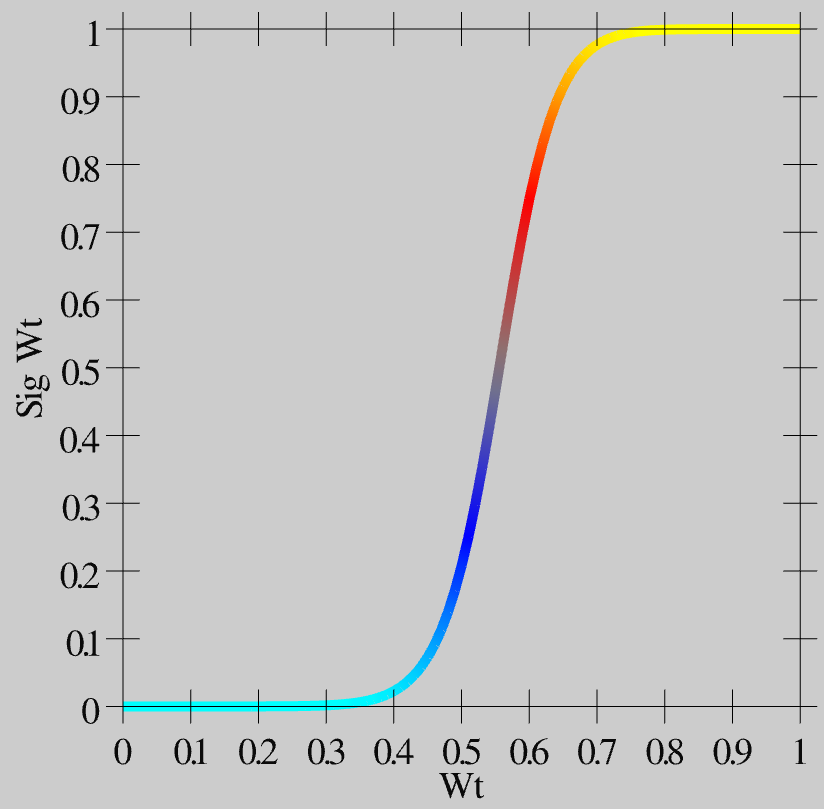
Weight contrast enhancement function, gain (gamma) = 6, offset (theta) = 1.25.

As you can see in [@fig:fig-wt-contrast-sigmoid-fun], this function creates greater contrast for weight values around this .5 central value — they get pushed up or down to the extremes. This contrast-enhanced weight value is then used for communication among the neurons, and is what shows up as the wt value in the simulator.

Biologically, we think of the plain weight value w, which is involved in the learning functions, as an internal variable that accurately tracks the statistics of the learning functions, while the contrast-enhanced weight value is the actual synaptic efficacy value that you measure and observe as the strength of interaction among neurons. Thus, the plain w value may correspond to the phosphorylation state of CAMKII or some other appropriate internal value that mediates synaptic plasticity.

Finally, see the Leabra Details Appendix for a few implementational details about the way that the time averages are computed, which don’t affect anything conceptually, but if you really want to know exactly what is going on..

When, Exactly, is there an Outcome that should Drive Learning?

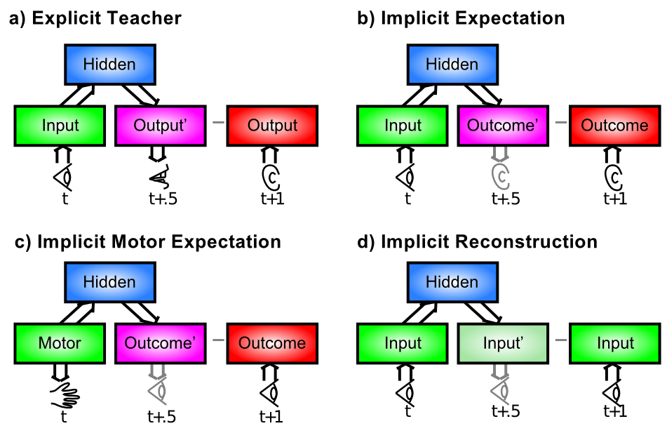
This is the biggest remaining question for error-driven learning. You may not have even noticed this issue, but once you start to think about implementing the XCAL equations on a computer, it quickly becomes a major problem. We have talked about how the error-driven learning reflects the difference between an outcome and an expectation, but it really matters that the short-term average activation representing the outcome state reflects some kind of actual outcome that is worth learning about. [@fig:fig-expect-outcome-errs] illustrates four primary categories of situations in which an outcome state can arise, which can play out in myriad ways in different real-world situations.

In our most recent framework described briefly above [@OReillyWyatteRohrlich17], the expectation-outcome timing is specified in terms of the 100 msec alpha trial. And within this trial, the combined circuitry between the deep neocortical layers and the thalamus end up producing an outcome state that drives predictive auto-encoder learning, which is basically the last case (d) in [@fig:fig-expect-outcome-errs], with an extra twist that during every 100 msec alpha trial, the network attempts to predict what will happen in the next 100 msec — the predictive aspect of the auto-encoder idea. Specifically, the deep layers attempt to predict what the bottom-up driven activity pattern over the thalamus will look like in the final plus-phase quarter of the alpha trial, based on activations present during the prior alpha trial. Because of the extensive bidirectional connectivity between brain areas, the cross-modal expectation / output sequence shown in panel (b) of [@fig:fig-expect-outcome-errs] is also supported by this mechanism. A later revision of this text will cover these ideas in more detail. Preliminary versions are available: [@OReillyWyatteRohrlich17; @KachergisWyatteOReillyEtAl14].

Another hypothesis for something that “marks” the presence of an important outcome is a phasic burst of a neuromodulator like dopamine. It is well established that dopamine bursts occur when an unexpected outcome arises, at least in the context of expectations of reward or punishment (we’ll discuss this in detail in the Motor Control and Reinforcement Learning Chapter. Furthermore, we know from a number of studies that dopamine plays a strong role in modulating synaptic plasticity. Under this hypothesis, the cortical network is always humming along doing standard BCM-like self-organizing learning at a relatively low learning rate (due to a small lambda parameter in the combined XCAL equation, which presumably corresponds to the rate of synaptic plasticity associated with the baseline tonic levels of dopamine), and then, when something unexpected occurs, a dopamine burst drives stronger error-driven learning, with the immediate short-term average “marked” by the dopamine burst as being associated with this important (salient) outcome. The XCAL learning will automatically contrast this immediate short-term average with the immediately available medium-term average, which presumably reflects an important contribution from the prior expectation state that was just violated by the outcome.

There are many other possible ideas for how the time for error-driven learning is marked, some of which involve local emergent dynamics in the network itself, and others that involve other neuromodulators, or networks with broad connectivity to broadcast an appropriate “learn now” signal. From everything we know about the brain, there are likely several such learning signals, each of which being useful in some particular subset of situations. This is an active area of ongoing research.

The Leabra Framework

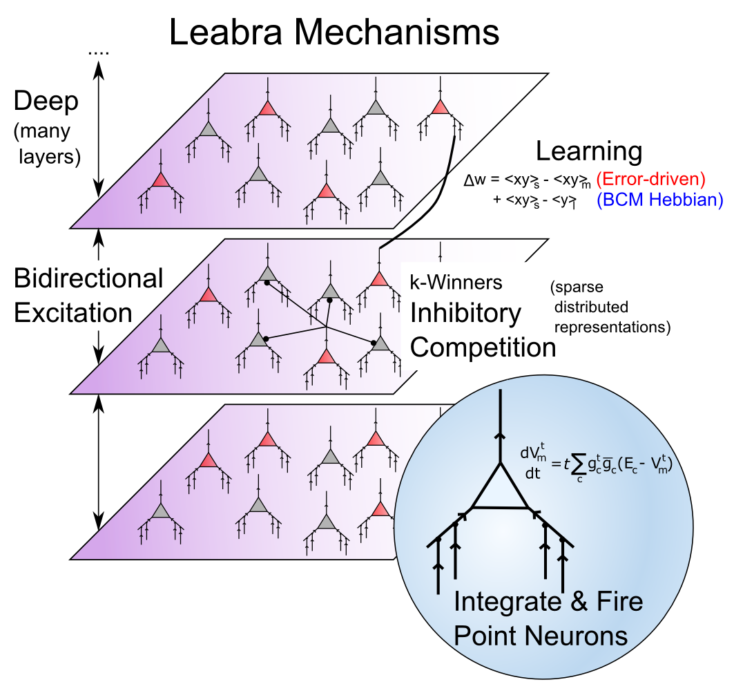
Summary of all the mechanisms in the Leabra framework used in this text, providing a summary of the last three chapters.

[@fig:fig-leabra-mechs-xcal] provides a summary of the Leabra framework, which is the name given to the combination of all the neural mechanisms that have been developed to this point in the text. Leabra stands for Learning in an Error-driven and Associative, Biologically Realistic Algorithm — the name is intended to evoke the “Libra” balance scale, where in this case the balance is reflected in the combination of error-driven and self-organizing learning (“associative” is another name for Hebbian learning). It also represents a balance between low-level, biologically-detailed models, and more abstract computationally-motivated models. The biologically-based way of doing error-driven learning requires bidirectional connectivity, and the Leabra framework is relatively unique in its ability to learn complex computational tasks in the context of this pervasive bidirectional connectivity. Also, the FFFB inhibitory function producing k-Winners-Take-All dynamics is unique to the Leabra framework, and is also very important for its overall behavior, especially in managing the dynamics that arise with the bidirectional connectivity.

The different elements of the Leabra framework are therefore synergistic with each other, and as we have discussed, highly compatible with the known biological features of the neocortex. Thus, the Leabra framework provides a solid foundation for the cognitive neuroscience models that we explore in Part II.

Exploration of Leabra

Open the family_trees simulation in CCN Sims to explore Leabra learning in a deep multi-layered network running a more complex task with some real-world relevance. This simulation is very interesting for showing how networks can create their own similarity structure based on functional relationships, refuting the common misconception that networks are driven purely by input similarity structure.

Appendix

Here are all the sub-topics within the Learning chapter, collected in one place for easy browsing. These may or may not be optional for a given course, depending on the instructor’s specifications of what to read:

Detailed Biology of Learning: more in-depth treatment of postsynaptic signaling cascades that mediate LTP and LTD, described in context of the [@UrakuboHondaFroemkeEtAl08] model of synaptic plasticity.
Hebbian Learning: extensive treatment of computational properties of Hebbian learning — starts with a simple manual simulation of Hebbian learning showing exactly how and why it captures patterns of co-occurrence.
Backpropagation: history and mathematical derivation of error-driven learning functions — strongly recommended to obtain greater insight into the computational nature of error-driven learning (starts with some important conceptual points before getting into the math).
Leabra Details: contains misc implementational details about the learning mechanisms, including how time averaged activations are computed.
Full set of Leabra equations on emergent leabra site.

Detailed Biology of Learning

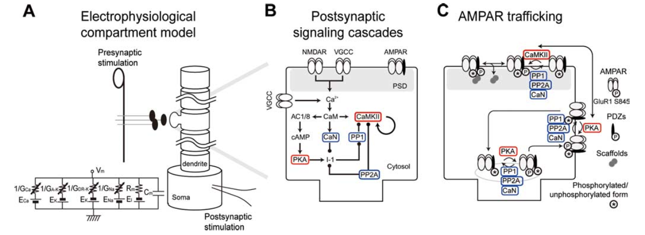
$Diagram of full set of steps involved in synaptic plasticity, including kinases driven by $Ca^{++}$ binding, and the effect they have on AMPA receptor expression in the synapse. Reproduced from Urakubo et al, 2008$

[@fig:fig-urakubo-et-al-model] shows a full set of chemical processes that are triggered by $Ca^{++}$ influx, and result in changes in AMPA receptor expression in the synapse. This figure is from the very detailed computational model by [@UrakuboHondaFroemkeEtAl08], which is highly recommended reading for those interested in the time course and dynamics of these chemical processes.

The Urakubo et al. (2008) model was constructed in a very “bottom up” fashion, by building in detailed chemical rate parameters and diffusion constants, etc, based on empirical measurements, for all of the major biological processes involved in synaptic plasticity. Having built this model, they found that it did not capture the classic spike timing dependent plasticity (STDP) curve, when driven by the exact STDP pairwise induction protocol (see figure of this in the main chapter text). However, by changing one aspect of the way the NMDA receptors function (adding what is known as an allosteric mechanism, where the NMDA receptor functions differently depending on binding by a substance called calmodulin), they were able to capture not only pairwise STDP, but also the weight changes that result from more complex patterns of spiking, in triplet and quadruplet experiments. Furthermore, they accurately capture the effects of changing the timing parameters on pairwise STDP experiments (e.g., interval between pairwise spikes, and number of repetitions thereof).

Thus, this model represents a remarkable bridge between detailed biological mechanisms, and the overall synaptic plasticity that results in actual experiments. Either this is a fantastic coincidence, or this model has managed to capture a reasonable chunk of the critical mechanisms of synaptic plasticity. We adopt the later view, and therefore leverage this model as a basis for our computational models described in the main chapter.

$Fit of the Urakubo et al. (2008) model with a simple learning function driven by the product of the total sending and receiving neural activity (frequency of firing in Hertz (Hz) times duration of firing in milliseconds). This simple linear function (called the ''XCAL dWt function'') can capture a considerable amount of the regularity present in the behavior of the Urakubo et al. (2008) model, with a correlation value of ''r=0.894''. The top portion of the figure shows graphs of three different sending Hz, with the X (horizontal) axis being the receiving unit Hz, Z (depth) is the duration of activity in fractions of a second (.1 to 1), and Y (vertical) is net change in synaptic weight. The black lines are the measured results from Urakubo et al. (2008), and the red are the values computed from the simple piecewise-linear function shown at the bottom of the figure.$

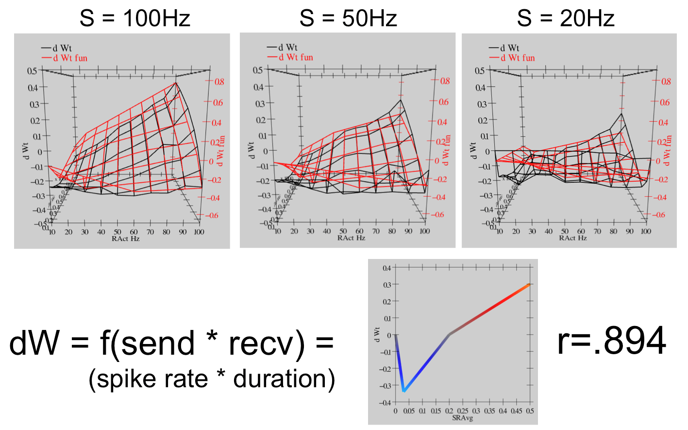
For the bottom-up derivation of XCAL, we systematically subjected the biologically detailed Urakubo et al. (2008) model to a range of different pre and post spike trains, with durations from 100 msec to a second, and spike rates from 10 to 100 Hz (Hertz or spikes per second). We then tried to fit the pattern of weight changes that resulted using a piecewise linear function of some form. [@fig:fig-xcal-dwt-fun-urakubo-fit-full] shows the results. The resulting function is shown at the bottom of the figure — if you compare with [@fig:fig-xcal-dwt-fun], you should see that this is essentially the qualitative shape of the function relating weight change to level of $Ca^{++}$. The top part of the figure is probably too complex to parse very well, but you should get the general impression that the red lines (generated by the piecewise linear function) fit the black lines (data from the Urakubo et al. (2008) model) pretty well. The correlation value of .894 represents a very good fit of the function to the data.

Thus, we are able to capture much of the incredible complexity of the Urakubo et al. (2008) model (and by extension, hopefully, the complexity of the actual synaptic plasticity mechanisms in the brain) using an extremely simple function. This is a very powerful simplification. But what does it mean?

First, the main input into this function is the total synaptic activity reflecting the firing rate and duration of activity of the sending and receiving neurons. In mathematical terms for a rate-code model with sending activity rate x and receiving activity rate y, this would just be the “Hebbian” product we described above: $\Delta w = f_{xcal} \left( x y, \theta_p\right)$ Where $f_{xcal}$ is the piecewise linear function shown in [@fig:fig-xcal-dwt-fun-urakubo-fit-full] or 4.4, which we can call the XCAL dWt function. It also takes an additional dynamic parameter $\theta_p$, which determines the point at which it crosses over from negative to positive weight changes — we’ll discuss this at length in a moment. Just for kicks, here is the mathematical expression of this function: $f_{xcal}(xy, \theta_p) = \left\{ \begin{array}{ll} (xy - \theta_p) & \mbox{if} \; xy > \theta_p \theta_d \\ -xy (1 - \theta_d) / \theta_d & \mbox{otherwise} \end{array} \right.$ where $\theta_d = .1$ is a constant that determines the point where the function reverses back toward zero within the weight decrease regime — this reversal point occurs at $\theta_p \theta_d$, so that it adapts according to the dynamic $\theta_p$ value.

As noted in the main chapter, the dependence of the NMDA channel on activity of both sending and receiving neurons can be summarized with this simple Hebbian product, and the level of $Ca^{++}$ is likely to reflect this value. Thus, the XCAL dWt function makes very good sense in these terms: it reflects the qualitative nature of weight changes as a function of $Ca^{++}$ that has been established from empirical studies and postulated by other theoretical models for a long time. When realistic spike trains with many spikes drive the complex synaptic plasticity mechanisms, this fundamental function emerges.

As a learning function, this basic XCAL dWt function has some advantages over a plain Hebbian function, while sharing its basic nature due to the “pre * post” term at its core. For example, because of the shape of the dWt function, weights will go down as well as up, whereas the Hebbian function only causes weights to increase. But it still has the problem that weights will increase without bound, and we’ll see in the next section that some other top-down computationally-motivated modifications can result in a much more powerful form of learning.

Hebbian Learning

This subsection provides a detailed treatment of Hebbian learning and popular variants thereof.

$Simple Hebbian learning demonstration across 4 time steps (t=0 thru 3). Bottom row of network has 3 input units, the last of which fires in an ''uncorrelated'' fashion with the other two. They all start out with weights w = .1. Receiving activity is just a linear sum of the sending activations times weights: $y = \sum x w = .1$ for the first time step. Learning is simple Hebbian: $\Delta w = xy$. As you fill in the remainder of the activations, weights, and weight changes, you will find that the two correlated input units dominate the receiving unit activation, and thus they end up being correlated in their activity, causing their weights to always increase. The third unit sometimes goes up and sometimes down, with no net increase over time. Thus, Hebbian learning discovers correlations in the inputs.$

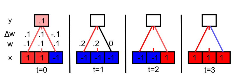
[@fig:fig-hebb-demo-blank] shows a simple demonstration of how Hebbian learning causes the receiving network to discover correlations in the patterns of input unit activation. The input units that are correlated end up dominating the receiving unit activity, and thus the receiving unit ends up being correlated with this subset of correlated inputs, and their weights always increase under the Hebbian learning function. Uncorrelated inputs bounce around without a systematic trend. If you keep going, you’ll see that the weights grow quickly without bound, so this is not a practical learning function, but it illustrates the essence of Hebbian learning.

Next, we do some math to show that the simplest version of Hebbian correlational learning, in the case of a single linear receiving unit that receives input from a set of input units, result in the unit extracting the first principle component of correlation in the patterns of activity over the input units.

Because it is linear, the receiving unit’s activation function is just the weighted sum of its inputs $y_j = \sum_k x_k w_{kj}$ where $k$ (rather than the usual $i$) indexes over input units, for reasons that will become clear (and all of the variables are a function of the current time step $t$ reflecting different inputs). The weight change is: $\Delta_t w_{ij} = \epsilon x_i y_j$ where $\epsilon$ is the learning rate and $i$ is the index of a particular input unit, and weights just increment these changes over time: $w_{ij}(t+1) = w_{ij}(t) + \Delta_t w_{ij}$

To understand the aggregate effects of learning over many patterns, we can just sum the changes over time: $\Delta w_{ij} = \epsilon \sum_t x_i y_j$ and we assume that $\epsilon = 1 / N$, where $N$ is the total number of patterns in the input. This turns the sum into an average: $\Delta w_{ij} = \langle x_i y_j \rangle_t$

Next, substitute into this equation the formula for $y_j$, showing that the weight changes are a function of the correlations between the input units: $\Delta w_{ij} = \langle x_i \sum_k x_k w_{kj} \rangle_t$ $= \sum_k \langle x_i x_k \rangle_t \langle w_{kj} \rangle_t$ $= \sum_k \mathbf{C}_{ik} \langle w_{kj} \rangle_t$

This new variable $\mathbf{C}{ik}$ is an element of the *correlation matrix* between the two input units $i$ and $k$, where correlation is defined here as the expected value (average) of the product of their activity values over time ($\mathbf{C}{ik} = \langle x_i x_k \rangle_t$). You might be familiar with the more standard correlation measure: $\mathbf{C}_{ik} = \frac{\langle (x_i - \mu_i)(x_k - \mu_k) \rangle_t} {\sqrt{\sigma^2_i \sigma^2_k}}$ which subtracts away the mean values ($\mu$) of the variables before taking their product, and normalizes the result by their variances ($\sigma^2$). Thus, an important simplification in this form of Hebbian correlational learning is that it assumes that the activation variables have zero mean and unit variance.

The implication of all this is that where strong correlations exist across input units, the weights for those units will increase because this average correlation value will be relatively large. Interestingly, if we run this learning rule long enough, the weights will become dominated by the strongest set of correlations present in the input, with the gap between the strongest set and the next strongest becoming increasingly large. Thus, this simple Hebbian rule learns the first (strongest) principal component of the input data.

One problem with the simple Hebbian learning rule is that the weights become infinitely large as learning continues. One solution to this problem was proposed by [@Oja82], known as subtractive normalization: $\Delta w_{ij} = \epsilon (x_i y_j - y^2_j w_{ij})$ As we did in Chapter 2, you just set the equation equal to zero and solve for the equilibrium or asymptotic weight values: $0 = \epsilon(x_i y_j - y^2_j w_{ij})$ $w_{ij} = \frac{ x_i}{y_j}$ $w_{ij} = \frac{ x_i}{\sum_k x_k w_{kj}}$

Thus, the weight from a given input unit will end up representing the proportion of that input’s activation relative to the total weighted activation over all the other inputs. This will keep the weights from growing without bound. Finally, because it is primarily based on the same correlation terms $\mathbf{C}_{ik}$ as the previous simple Hebbian learning rule, this Oja rule still computes the first principal component of the input data (though the proof of this is somewhat more involved, see [@HertzKroghPalmer91] for a nice treatment).

Moving beyond a single hidden unit, there are ways of configuring inhibition so that the units end up learning the sequence of PCA values of the correlation matrix in eigenvalue order [@Sanger89; @Oja89]. In [@OReillyMunakata00], we developed a different alternative known as conditional principal components analysis or CPCA, which assumes that we want the weights for a given input unit to represent the conditional probability that the input unit ($x_i$) was active given that the receiving unit ($y_j$) was also active: $w_{ij} = P(x_i = 1 | y_j = 1)$ $w_{ij} = P(x_i | y_j)$ where the second form uses simplified notation that will continue to be used below.

The important characteristic of CPCA is that the weights will reflect the extent to which a given input unit is active across the subset of input patterns represented by the receiving unit (i.e., conditioned on this receiving unit). If an input pattern is a very typical aspect of such inputs, then the weights from it will be large (near 1), and if it is not so typical, they will be small (near 0).

Following the analysis of [@RumelhartZipser85], the CPCA learning rule can be derived as: $\Delta w_{ij} = \epsilon [y_j x_i - y_j w_{ij}]$ $= \epsilon y_j (x_i - w_{ij})$ The two equivalent forms of this equation are shown to emphasize the similarity of this learning rule to Oja’s normalized PCA learning rule, while also showing its simpler form, which emphasizes that the weights are adjusted to match the value of the sending unit activation $x_i$ (i.e., minimizing the difference between $x_i$ and $w_{ij}$), weighted in proportion to the activation of the receiving unit ($y_j$).

We use the expression $P(y_j	t)$ to represent the probability that the receiving unit $y_j$ is active given that some particular input pattern $t$ was presented. $P(x_i	t)$ represents the corresponding thing for the sending unit $x_i$. Substituting these into the learning rule, the total weight update computed over all the possible patterns $t$ (and multiplying by the probability that each pattern occurs, $P(t)$) is:
$$ \Delta w_{ij} = \epsilon \sum_t [P(y_j	t) P(x_i	t) - P(y_j	t) w_{ij}] P(t) $$
$$ = \epsilon \left( \sum_t P(y_j	t) P(x_i	t) P(t) - \sum_t P(y_j	t) P(t) w_{ij} \right) $$

As usual, we set $\Delta w_{ij}$ to zero and solve: $w_{ij} = \frac{\sum_t P(y_j | t) P(x_i | t) P(t)} {\sum_t P(y_j | t) P(t)}$ Interestingly, the numerator is the definition of the joint probability of the sending and receiving units both being active together across all the patterns $t$, which is just $P(y_j, x_i)$. Similarly, the denominator gives the probability of the receiving unit being active over all the patterns, or $P(y_j)$. Thus, we can rewrite the preceding equation as: $w_{ij} = \frac{P(y_j, x_i)}{P(y_j)}$ $w_{ij} = P(x_i | y_j)$ at which point it becomes clear that this fraction of the joint probability over the probability of the receiver is just the definition of the conditional probability of the sender given the receiver.

Although CPCA is effective and well-defined mathematically, it suffers one major problem relative to the BCM formulation that we now use: it drives significant LTD (weight decrease) when a sending neuron is not active, and the receiving unit is active. This results in a significant amount of interference of learning across time. By contrast, the XCAL dWt function specifically returns to zero when either sending or receiving neuron has zero activity, and that significantly reduces interference, preserving existing weight values for inactive neurons.

Backpropagation

In this subtopic, we trace the mathematical progression of error-driven learning from a simple two-layer network, which was developed in 1960, to a network with three or more layers, which took 26 years to be invented for the last time (several others invented it earlier, but it didn’t really catch on). In the process, we develop a much more rigorous understanding of what error-driven learning is, which can also be applied directly to understanding what the XCAL learning function in its error-driven mode is doing. We start off with a high-level conceptual summary, working backward from XCAL, that should be accessible to those with a basic mathematical background (requiring only basic algebra), and then get progressively more into the math, where we take advantage of concepts from calculus (namely, the notion of a partial derivative).

The highest-level summary is that XCAL provides a very good approximation to an optimal form of error-driven learning, called error backpropagation, which works by directly minimizing a computed error statistic through steepest gradient descent. In other words, backpropagation is mathematically designed to learn whatever you throw at it in the most direct way possible, and XCAL basically does the same thing. If you want to first understand the principled math behind backpropagation, skip down to read the Gradient Descent on Error and the Delta Rule section below, and then return here to see how XCAL approximates this function.

The critical difference is that XCAL uses bidirectional activation dynamics to communicate error signals throughout the network, whereas backpropagation uses a biologically implausible procedure that propagates error signals backward across weight values, in the opposite direction of the way that activation typically flows (hence the name). As discussed in the main chapter, the XCAL network experiences a sequence of activation states, going from an expectation to experiencing a subsequent outcome, and learns on the difference between these two states. In contrast, backpropagation computes a single error delta value that is effectively the difference between the outcome and the expectation, and then sends this single value backwards across the weights. In the following math, we show how these two ways of doing error-driven learning are approximately equivalent.

The primary value of this exercise is to first establish that XCAL can perform a powerful, effective form of error-driven learning, and also to obtain further insights into the essential character of this error-driven learning by understanding how it is derived from first principles. One of the most important intuitive ideas that emerges from this analysis is the notion of credit assignment — you are encouraged to read up through that section.

To begin, the error-driven aspect of XCAL is effectively: $\Delta w \approx \langle xy \rangle_s - \langle xy \rangle_m$ which reflects a contrast between the average firing rate during the outcome, represented by the first term, and that over the expectation, represented by the second term.

We will see how this XCAL rule is related to the backpropagation error-minimizing rule, but achieves this function in a more biologically constrained way. This was the same goal of previous attempts including the GeneRec (generalized recirculation) algorithm [@OReilly96], which is equivalent to the Contrastive Hebbian Learning (CHL) equation [@MovellanMcClelland93]: $\Delta w = \left(x^+ y^+\right) - \left(x^- y^-\right)$ Here, the first term is the activity of the sending and receiving units during the outcome (in the plus phase), while the second term is the activity during the expectation (in the minus phase). CHL is so-named because it involves the contrast or difference between two Hebbian-like terms. As you can see, XCAL is essentially equivalent to CHL, despite a few differences:

XCAL actually uses the XCAL dWt function instead of a direct subtraction, which causes weight changes to go to 0 when short term activity is 0 (as dictated by the biology).
XCAL is based on average activations across the entire evolution of attractors (reflected by accumulated $Ca^{++}$ levels), instead of based on single points of activation (i.e., the final attractor state in each of two phases, as used somewhat unrealistically in CHL — how would the plasticity rules ‘know’ exactly what counts as the final state of each phase?).

For the present purposes, we can safely ignore these factors, which allows us to leverage all of the analysis that went into understanding GeneRec — itself a large step towards biological plausibility relative to backpropagation.

The core of this analysis revolves around the following simpler version of the GeneRec equation, which we call the GeneRec delta equation: $\Delta w = x^- \left(y^+ - y^- \right)$ where the weight change is driven only by the delta in activity on the receiving unit y between the plus (outcome) and minus (expectation) phases, multiplied by the sending unit activation x. One can derive the full CHL equation from this simpler GeneRec delta equation by adding a constraint that the weight changes computed by the sending unit to the receiving unit be the same as those of the receiving unit to the sending unit (i.e., a symmetry constraint based on bidirectional connectivity), and by replacing the minus phase activation for the sending unit with the average of the minus and plus phase activations (which ends up being equivalent to the midpoint method for integrating a differential equation). You can find the actual derivation later in the section GeneRec and Activation Differences, but you can take our word for it for the time being.

This equation has the desired property of credit assignment: the weight change is proportional to $ x^- $, which reflects how much this sender contributed to the error being learned from.

Interestingly, the GeneRec delta equation is equivalent in form to the delta rule, which we derive below as the optimal way to reduce error in a two layer network (input units sending to output units, with no hidden units in between). The delta rule was originally derived by [@WidrowHoff60], and it is also basically equivalent to a gradient descent solution to linear regression.

But two-layer networks are very limited in what they can compute. As we discussed in the Networks Chapter, you really need those hidden layers to form higher-level ways of re-categorizing the input, to solve challenging problems (you will also see this directly in the simulation explorations in this chapter). As we discuss more below, the limitations of the delta rule and two-layer networks were highlighted in a very critical paper by [@MinskyPapert69], which brought research in the field of neural network models nearly to a standstill for nearly 20 years.

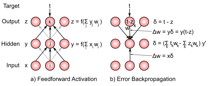
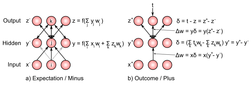
In 1986, David Rumelhart and colleagues [@RumelhartHintonWilliams86] published a landmark paper on the backpropagation learning algorithm, which essentially extended the delta rule to networks with three or more layers ([@fig:fig-generec-compute-delta]). These models have no limitations on what they can learn, and they opened up a huge revival in neural network research, with backpropagation neural networks providing practical and theoretically interesting solutions to a very wide range of problems.

The essence of the backpropagation (also called “backprop”) algorithm is captured in this delta backpropagation equation: $\Delta w = x \left( \sum_k \delta_k w_k \right) y'$ where x is again the sending activity value, $\delta$ is the error derivative for the units in the next layer above the layer containing the current receiving unit y (with each such unit indexed by the subscript k), and $w_k$ is the weight from the receiving unit y to the k’th such unit in the next layer above (see [@fig:fig-bp-compute-delta]). Ignore the $y’$ term for the time being — it is the derivative of the receiving unit’s activation function, and it will come in handy in a bit.

So we’re propagating this “delta” (error) value backward across the weights, in the opposite direction that the activation typically flows in the “feedforward” direction, which is from the input to the hidden to the output (backprop networks are typically feedforward, though bidirectional versions have been developed as discussed below). This is the origin of the “backpropagation” name.

Before we unpack this equation a bit more, let’s consider what happens at the output layer in a standard three-layer backprop network like that pictured in the Figure. In these networks, there is no outcome/plus phase, but instead we just compare the output activity of units in the output layer (effectively the expectation) and compute externally the difference between these activities and the target activity values t. The difference is the delta value: $\delta = t - z$ and is used to drive learning by changing the weight from sending unit y in the hidden layer to a given output unit z is: $\Delta w = y \delta = y (t - z)$ You should recognize that this is exactly the delta rule as described above (where we keep in mind that y is now a sending activation to the output units). The delta rule is really the essence of all error-driven learning methods.

Now let’s get back to the delta backpropagation equation, and see how we can get from it to GeneRec (and thus to XCAL). We just need to replace the $\delta_k$ term with the value for the output units, and then do some basic rearranging of terms, and we get very close to the GeneRec delta equation: $\Delta w = x \left( \sum_k (t_k - z_k) w_k \right) y'$ $\Delta w = x \left( \sum_k t_k w_k - \sum_k z_k w_k \right) y'$ If you compare this last equation with the GeneRec delta equation, they would be equivalent (except for the y’ term that we’re still ignoring) if we made the following definitions: $y^+ = \left. \sum_k t_k w_k \right.$ $y^- = \left. \sum_k z_k w_k \right.$ $x^- = x$ Interestingly, these sum terms are identical to the net input that unit y would receive from unit z if the weight went the other way, or, critically, if y also received a symmetric, bidirectional connection from z, in addition to sending activity to z. Thus, we arrive at the critical insight behind the GeneRec algorithm relative to the backpropagation algorithm:

Symmetric bidirectional connectivity can convey error signals as the difference between two activity states (plus/outcome vs. minus/expectation), instead of sending a single “delta” error value backward down a single weight in the opposite (backpropagation) direction.

The only wrinkle in this argument at this point is that we had to assign the activation states of the receiving unit to be equal to those net-input like terms (even though we use non-linear thresholded activation functions), and also those net input terms ignore the other inputs that the receiving unit should also receive from the sending units in the input layer. The second problem is easily dispensed with, because those inputs from the input layer would be common to both “phases” of activation, and thus they cancel out when we subtract $y^+ - y^-$. The first problem can be solved by finally no longer ignoring the y’ term — it turns out that the difference between a function evaluated at two different points can be approximated as the difference between the two points, times the derivative of the function: $f(a) - f(b) \approx f'(a) (a-b)$ So we can now say that the activations states of y are a function of these net input terms: $y^+ = f \left( \sum_k t_k w_k \right)$ $y^- = f \left( \sum_k z_k w_k \right)$ and thus their difference can be approximated by the difference in net inputs times the activation function derivative: $y^+ - y^- \approx y' \left( \sum_k t_k w_k - \sum_k z_k w_k \right)$ Which gets us right back to the GeneRec delta equation as being a good approximation to the delta backpropagation equation: $\Delta w = x^- \left(y^+ - y^- \right) \approx x \left( \sum_k \delta_k w_k \right) y'$

So if you’ve followed along to this point, you can now rest easy by knowing that the GeneRec (and thus XCAL) learning functions are actually very good approximations to error backpropagation. As we noted at the outset, XCAL uses bidirectional activation dynamics to communicate error signals throughout the network, in terms of averaged activity over two distinct states of activation (expectation followed by outcome), whereas backpropagation uses a biologically implausible procedure that propagates a single error value (outcome - expectation) backward across weight values, in the opposite direction of the way that activation typically flows.

Gradient Descent on Error and the Delta Rule

Now, we’ll back up a bit and trace more of a historical trajectory through error-driven learning, starting by deriving the delta rule through the principle of steepest gradient descent on an error function. To really understand the mathematics here, you’ll need to understand calculus and the notion of a derivative. Interestingly, we only need the most basic forms of derivatives to do this math — it really isn’t very fancy. The basic strategy is to define an error function which tells you how poorly your network is doing at a task, and then take the negative of the derivative of this error function relative to the synaptic weights in the network, which then tells you how to adjust the synaptic weights so as to minimize error. This is what error-driven learning does, and mathematically, we take the simplest, most direct approach.

A very standard error function, commonly used in statistics, is the sum squared error (SSE): $SSE = \sum_k \left( t_k - z_k \right)^2$ which is the sum over output units (indexed by k) of the target activation t minus the actual output activation that the network produced (z), squared. There is typically an extra sum here too, over all the different input/output patterns that the network is being trained on, but it cancels out for all of the following math, so we can safely ignore it.

In the context of the expectation and outcome framework of the main chapter, the outcomes are the targets, and the expectations are the output activity of the network.

For the time being, we assume a linear activation function of activations from sending units y, and that we just have a simple two-layer network with these sending units projecting directly to the output units: $z_k = \left. \sum_j y_j w_{jk} \right.$

Taking the negative of the derivative of SSE with respect to the weight w, which is more easily computed by breaking it down into two parts using the chain rule to first get the derivative of SSE with respect to the output activation z, and multiplying that by the derivative of z with respect to the weight: $\Delta w_{jk} = -\frac{\partial SSE}{\partial w_{jk}} = -\frac{\partial SSE}{\partial z_k} \frac{\partial z_k}{\partial w_{jk}}$ $= 2 (t_k - z_k) y_j$

When you break down each step separately, it is all very straightforward: $\frac{\partial SSE}{\partial z_k} = -2 (t_k - z_k)$ $\frac{\partial z_k}{\partial w_{jk}} = y_j$ (the other elements of the sums drop out because the first partial derivative is with respect to $z_k$ so derivative for all other $z$’s is zero, and similarly the second partial derivative is with respect to $y_j$ so the derivative for the other $y$’s is zero.)

Thus, the negative of $\partial SSE / \partial w_{jk}$ is $2 (t_k -z_k)$ and since 2 is a constant, we can just absorb it into the learning rate parameter.

Breaking down the error-minimization in this way, it becomes apparent that the weight change should be adjusted in proportion to both the error (difference between the target and the output) and the extent to which the sending unit y was active. This modulation of weight change by activity of the sending unit achieves a critical credit assignment function (or rather blame assignment in this case), so that when an error is made at the output, weights should only change for the sending units that contributed to that error. Sending units that were not active did not cause the error, and their weights are not adjusted.

As noted above, the original delta rule was published by [@WidrowHoff60], followed by the critique by [@MinskyPapert69], showing that such models could not learn a large class of basic but nonlinear logical functions, for example the XOR function. XOR states that the output should be true (active) if either one of two inputs are true, but not both. This requires a strong form of nonlinearity that simply could not be represented by such models. In retrospect, it should have been obvious that the problem was the use of a two-layer network, but as often happens, this critique left a bad “odor” over the field, and people simply pursued other approaches (mainly symbolic AI, which Minsky was an advocate for).

Then, roughly 26 years later, David Rumelhart and colleagues published a paper on the backpropagation learning algorithm, which extended the delta-rule style error-driven learning to networks with three or more layers. The addition of the extra layer(s) now allows such networks to solve XOR and any other kind of problem (there are proofs about the universality of the learning procedure). The problem is that above, we only considered how to change weights from a sending unit y to an output unit z, based on the error between the target t and actual output activity. But for multiple stages of hidden layers, how do we adjust the weights from the inputs to the hidden units? Interestingly, the mathematics of this involves simply adding a few more steps to the chain rule.

First, we define the activation function in terms of $\eta_j$ as the net input to unit $j$, i.e., the product of sending activity $x_i$ and weights: $\eta_j = \sum x_i w_{ij}$

and then the unit activity is a function of this net input: $y_j = f(\eta_j)$

The goal is to again minimize the error (SSE) as a function of the weights, $\Delta w_{ij} = -\frac{\partial SSE}{\partial w_{ij}}$.

The chain rule expansion of the basic activation function through hidden units $j$ and output units $k$ is thus:

\[= -\frac{\partial SSE}{\partial z_k} \frac{\partial z_k}{\partial \eta_k} \frac{\partial \eta_k}{\partial y_j} \frac{\partial y_j}{\partial \eta_j} \frac{\partial \eta_j}{\partial w_{ij}}\]

Although this looks like a lot, it is really just applying the same chain rule as above repeatedly. To know how to change the weights from input unit $x_i$ to hidden unit $y_j$, we have to know how changes in this weight $w_{ij}$ are related to changes in the SSE. This involves computing how the SSE changes with output activity, how output activity changes with its net input, how this net input changes with hidden unit activity $y_j$, how in turn this activity changes with its net input $\eta_j$, and finally, how this net input changes with the weights from sending unit $x_i$ to hidden unit $y_j$. Once all of these factors are computed, they can be multiplied together to determine how the weight $w_{ij}$ should be adjusted to minimize error, and this can be done for all sending units to all hidden units (and also as derived earlier, for all hidden units to all output units).

We again assume a linear activation function at the output for simplicity, so that $\partial z_k / \partial \eta_k = 1$. We allow for non-linear activation functions in the hidden units y, and simply refer to the derivative of this activation function as $y’$ (which for the common sigmoidal activation functions turns out to be $y (1-y)$ but we leave it in generic form here so that it can be applied to any differentiable activation function. The solution to the above equation is then, applying each step in order, $-\frac{\partial SSE}{\partial w_{ij}} = \sum_k (t_k - z_k) * 1 * w_{jk} * y' * x_i$ $= x \left( \sum_k \delta_k w_{jk} \right) y'$ as specified earlier.

You can see that this weight change occurs not only in proportion to the error at the output, and the ‘backpropagated’ error at the hidden unit activity y, but also to the activity of the sending unit $x_i$. So, once again, the learning rule assigns credit/blame to change weights based on active input units that contributed to the error, weighted by the degree to the error at the level of hidden unit activities contribute to errors at the output (which is the weight $w_{jk}$). At all steps along the process, the appropriate units and weights are factored in to minimize errors. This procedure can be repeated for any arbitrary number of layers, with repeated application of the chain rule.

GeneRec and Activation Differences

Finally, we can derive GeneRec in full (see [@OReilly96] for more details). First reconsider the equation for the $\delta_j$ variable on the hidden unit in backpropagation: $\delta_j = - \sum_k (t_k - o_k) w_{jk} h_j(1-h_j)$ The main biological implausibility in this equation comes from the passing of the error information on the outputs backward, and the multiplying of this information by the feedforward weights and by the derivative of the activation function. There is simply no known biological way for such a signal to be transported backward like this [@Crick89].

We avoid the implausible error propagation procedure by converting the computation of error information multiplied by the weights into a computation of the net input to the hidden units. For mathematical purposes, we assume for the moment that our bidirectional connections are symmetric, or $w_{jk}=w_{kj}$. We will see later that the argument below holds even if we do not assume exact symmetry. With $w_{jk}=w_{kj}$: $\delta_j = - \sum_k (t_k - o_k) w_{jk} h_j(1-h_j)$ $= - \sum_k (t_k - o_k) w_{kj} h_j(1-h_j)$ $= - \left(\sum_k (t_k w_{kj}) - \sum_k (o_k w_{kj})\right) h_j(1-h_j)$ $= - (\eta^+_j - \eta^-_j) h_j(1-h_j)$

That is, $w_{kj}$ can be substituted for $w_{jk}$ and then this term can be multiplied through $(t_k - o_k)$ to get the difference between the net inputs to the hidden units (from the output units) in the two phases. Bidirectional connectivity thus allows error information to be communicated in terms of net input to the hidden units, rather than in terms of $\delta$s propagated backward and multiplied by the strength of the feedforward synapse.

Next, we can deal with the remaining $h_j(1-h_j)$ by applying the difference-of-activation-states approximation. $h_j(1-h_j)$ can be expressed as $\sigma’(\eta_j)$, the derivative of the activation function, so: $\delta_j = - (\eta^+_j - \eta^-_j) \sigma'(\eta_j)$ This product can be approximated by just the difference of the two sigmoidal activation values computed on these net inputs: $\delta_j \approx -(h^+_j - h^-_j)$ That is, the difference in a hidden unit’s activation values is approximately equivalent to the difference in net inputs times the slope of the activation function. This also has the benefit of implicitly computing the derivative of the activation function, so we can use more complex biologically-based ones without worrying about needing to compute their derivatives.

Once we have the $\delta$ terms for the hidden units computed as the difference in activation across the two phases, we end up with: $\Delta w_{ij} = - \epsilon \delta_j s_i = \epsilon (h^+_j - h^-_j) s^-_i$ Thus, through bidirectional connectivity and the approximation of the product of net input differences and the derivative of the activation function, hidden units implicitly compute the information needed to minimize error as in backpropagation, but using only locally available activity signals.

To get to CHL, we make two small but significant changes. First, there is a more sophisticated way of updating weights, known as the midpoint method, that uses the average of both the minus and plus phase activation of the sending unit $x_i$, instead of just the minus phase alone: $\Delta w_{ij} = \epsilon (y^+_j - y^-_j) \frac{x^-_i+x^+_i}{2}$

Second, the mathematical derivation of the learning rule depends on the weights being symmetric, and yet the basic GeneRec equation is not symmetric (i.e., the weight changes computed by unit $j$ from unit $i$ are not the same as those computed by unit $i$ from unit $j$). So, even if the weights started out symmetric, they would not likely remain that way under the basic GeneRec equation. Making the weight changes symmetric (the same in both directions) both preserves any existing weight symmetry, and, when combined with a small amount of weight decay [@Hinton89] and/or soft weight bounding, actually works to symmetrize initially asymmetric weights. A simple way of preserving symmetry is to take the average of the weight updates for the different weight directions: $\Delta w_{ij} = \epsilon \frac{1}{2} \left[ (y^+_j - y^-_j) \frac{(x^+_i + x^-_i)}{2} + (x^+_i - x^-_i) \frac{(y^+_j + y^-_j)}{2} \right]$ $= \epsilon \left[ x^+_i y^+_j -x^-_i y^-_j \right]$ (where the $1/2$ for averaging the weight updates in the two different directions gets folded into the arbitrary learning rate constant $\epsilon$). Because many terms end up canceling, the weight change rule that results is just the CHL equation as shown above.

Leabra Details

The full set of Leabra equations on emergent leabra site.

First, it turns out in practice that computing the average of the sending and receiving activations over the short time period: $\langle xy \rangle_s$ can be approximated by the computationally less expensive product of the averages: $\langle xy \rangle_s \approx \langle x \rangle_s \langle y \rangle_s = x_s y_s$ (the last expression is a convenient short-hand for expressing the short-term average of the relevant variables).

Thus, we separately compute these averages on each neuron, and then multiply the averages when it is time to compute synaptic weight changes — in contrast, computing the average of the product requires integrating the average at every synapse — there are typically many many more synapses than neurons, so this represents a significant computational savings. Furthermore, the learning results (i.e., the ability of networks to learn efficiently) are typically somewhat better computing these averages separately, for reasons that are not entirely clear at this point.

The default time constant for the long-term running-average activation value used as a floating threshold in the BCM learning rule is tau = 10, which means that it integrates over roughly 10 trials — this is fairly fast relative to some expectations of “long term”, but that does tend to work better computationally when combined with error-driven learning, to keep the floating threshold more fluid and responsive to the current state of the neuron. Better biological data is needed to pin down the appropriate constraints on this parameter, to see if this is biologically plausible or not.